Numerical Methods for Solving ODEs

Ordinary Differential Equations (ODEs):

• Equations which are composed of an unknown function and its derivatives are called differential equations.
• Differential equations play a fundamental role in engineering because many physical phenomena are best formulated mathematically in terms of their rate of change.

For example: the pendulum

$$F=ma⟹\frac{\mathrm{d}v}{\mathrm{d}t}=g-\frac{c}{m}v$$

• Analytical:

$$v=\frac{g}{mc}(1-c^{-(c/m)t})$$

• Numberical:

$$v_{i+1}=v_i+(g-\frac{c}{m}{v}_i)\mathrm{\Delta }t$$

Use of Taylor series

This lecture is devoted to solving ordinary differential equations of the form

$$\frac{\mathrm{d}y}{\mathrm{d}x}=f(x,y).$$

• Suppose that the solution passes through the point $(x_0,y_0)$
• we attempt, by a step-by-step method, to calculate successively approximate values of $y$ at the points $x_1=x_0+h,x_2=x_0+2h,\cdots ,x_k=x_0+kh\cdots$, where $h$ is a suitably chosen spacing along the $X$ axis
• Use the Taylor series representation in the form of function $y$ at $x$ point:

$$y(x+h)=y(x)+y^{\prime }(x)\frac{h}{1!}+y^{\prime \prime }(x)\frac{h^2}{2!}+\cdots$$

setting $x=x_k$, we obtain the formula:

$$y_{k+1}=y_k+y_k^{\prime }\frac{h}{1!}+y_k^{\prime \prime }\frac{h^2}{2!}+\cdots$$

where

$$\begin{array}{ll}{y}^{\prime }=F(x,y),& y_k^{\prime }=F(x_k,y_k)\\ y^{\prime \prime }=\frac{\partial F}{\partial x}+\frac{\partial F}{\partial y}\frac{\mathrm{d}y}{\mathrm{d}x},& y_k^{\prime \prime }=\frac{\partial F(x_k,y_k)}{\partial x}+\frac{\partial F(x_k,y_k)}{\partial y}{y}_k^{\prime }\end{array}$$

Example1

$$\frac{\mathrm{d}y}{\mathrm{d}x}=y-x.$$

• with the initial condition that $y=2$ at $x=0$.

$$\begin{array}{rl}& \frac{\mathrm{d}y}{\mathrm{d}x}-y=-x\\ ⟹& y=3\exp (x)-x-1.\end{array}$$

• Choose an interval $h=0.1$,
• calculate successively the approximate values of $y$ at $x=0.1,0.2,0.3$, and so on:

$$y^{\prime }=y-x,y^{\prime \prime }=y^{\prime }-1,y^{\prime \prime \prime }=y^{\prime \prime },\dots$$

• At $x=0$, with $k=0$

$$\begin{array}{rl}{y}_0^{\prime }& =2,y_0^{\prime \prime }=1,y_0^{\prime \prime \prime }=1,\cdots ,\\ y_1& =y{|}_{x=0.1}=y_0+2h+\frac{h^2}{2}+\frac{h^3}{6}+\cdots \\ & \cong 2+0.2000+0.0050+0.0002+\cdots =2.2052.\end{array}$$

$y{|}_{x=0.1}=3\exp (0.1)-0.1-1\approx 2.2155$

• At $x=0.1$, with $k=1$

$$\begin{array}{rl}{y}_1^{\prime }& \cong 2.1052,y_1^{\prime \prime }\cong 1.1052,y_1^{\prime \prime \prime }\cong 1.1052,\cdots ,\\ y_2& \cong y{|}_{x=0.2}=y_1+2.1052h+0.5526h^2+0.1842h^3+\cdots \\ & \cong 2.2052+0.2105+0.0055+0.0002+\cdots =2.4214.\end{array}$$

$y{|}_{x=0.2}=3\exp (0.2)-0.2-1\approx 2.4642$

Euler’s Methods

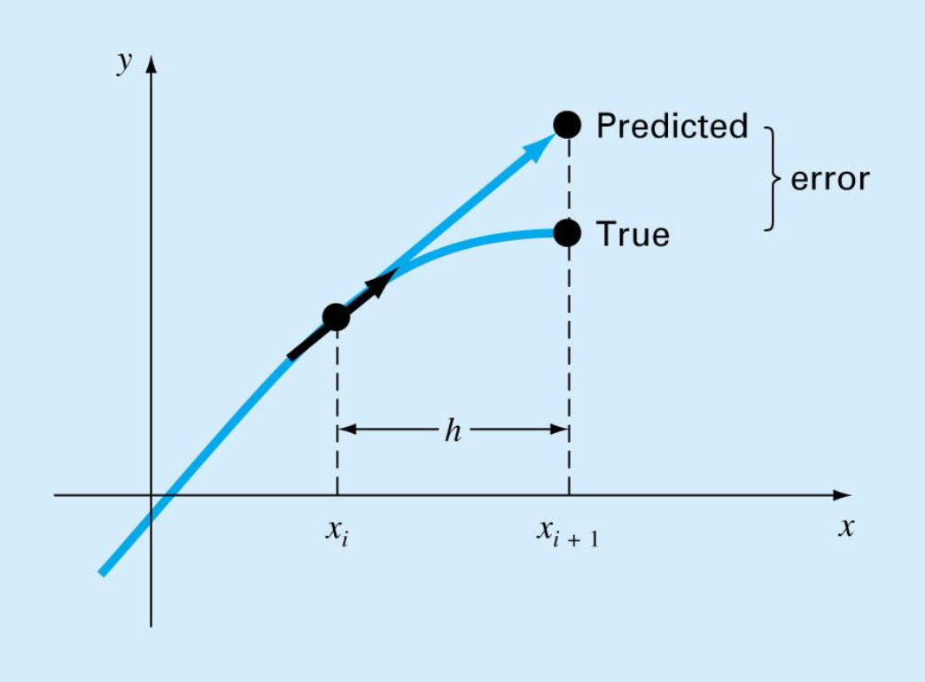
The first derivative provides a direct estimate of the slope at $x_i$:

$$\varphi =f(x_i,y_i).$$

where $f(x_i,y_i)$ is the differential equation evaluated at $x_i$ and $y_i$. This estimate can be substituted into the equation:

$$y_{i+1}=y_i+f(x_i,y_i)h$$

A new value of $y$ is predicted using the slope to extrapolate linearly over the step size $h$.

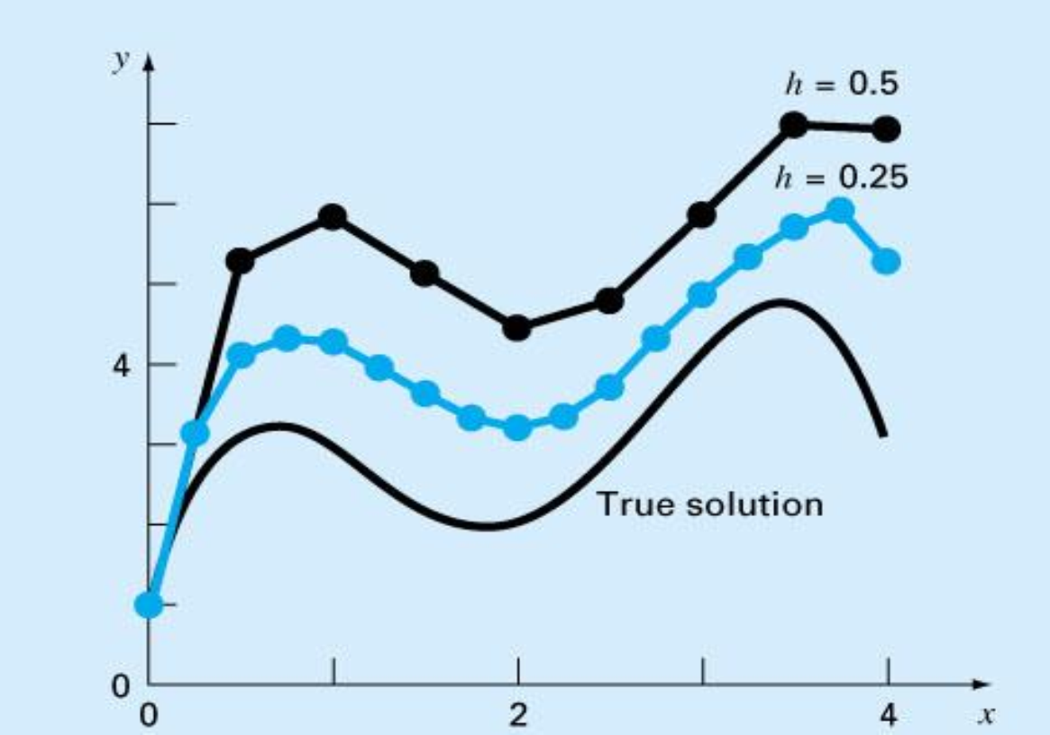
Error Analysis for Euler’s Method

Numerical solutions of ODEs involves two types of error:

• Truncation error
  • Local truncation error
  $$E_a=\frac{f^{\prime }(x_i,y_i)}{2!}{h}^2+\cdots =\frac{y^{″}(x_i,y_i)}{2!}{h}^2+O(h^3)=O(h^2)$$
  • Propagated truncation error
  • The sum of the two is the total or global truncation error
• Round-off errors

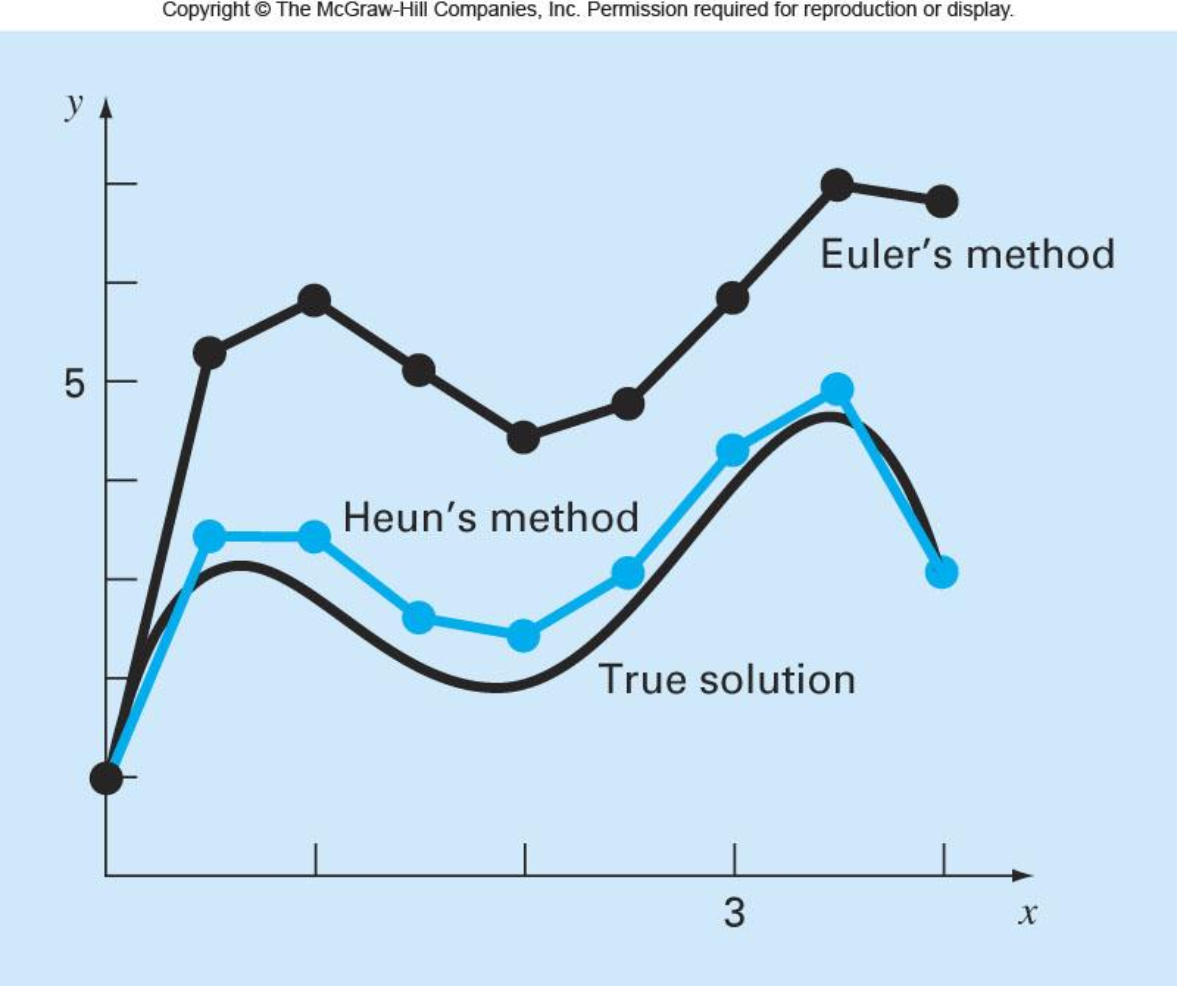
Improvements of Euler’s method

A fundamental source of error in Euler’s method is that the derivative at the beginning of the interval is assumed to apply across the entire interval.

Two simple modifications are available to circumvent this shortcoming:

• Heun’s Method
• The Midpoint (or Improved Polygon) Method

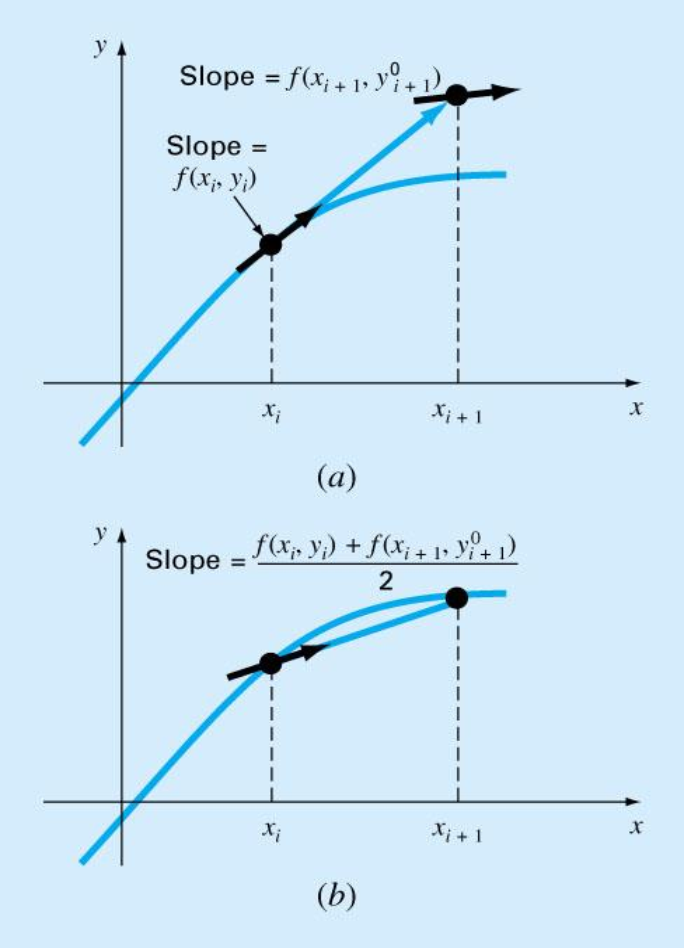
Heun’s Method

One method to improve the estimate of the slope involves the determination of two derivatives for the interval:

• At the initial point
• At the end point

The two derivatives are then averaged to obtain an improved estimate of the slope for the entire interval.

• Predictor:

$$y_{i+1}^0=y_i+f(x_i,y_i)h$$

• Corrector:

$$y_{i+1}=y_i+\frac{f(x_i,y_i)+f(x_{i+1},y_{i+1}^0)}{2}h$$

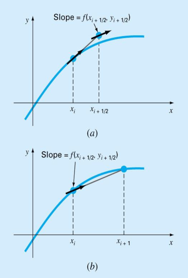
The Midpoint / Improved Polygon Method

Uses Euler’s method to predict a value of $y$ at the midpoint of the interval:

$$y_{i+1}=y_i+f(x_{i+1/2},y_{i+1/2})h$$

where

$$\begin{array}{rl}{x}_{i+1/2}& =x_i+\frac{1}{2}h\\ y_{i+1/2}& =y_i+f(x_i,y_i)\frac{h}{2}\end{array}$$

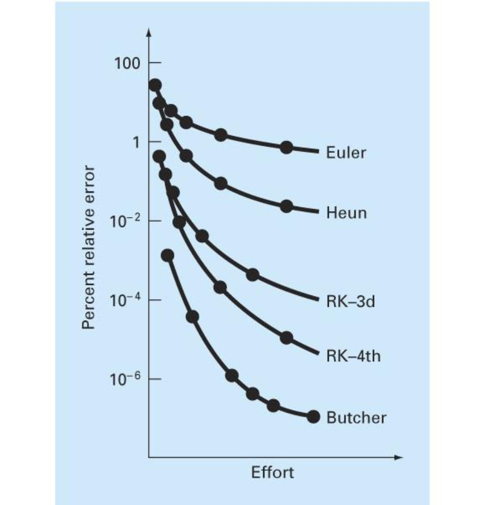
Runge-Kutta (RK) Methods

Runge-Kutta methods achieve the accuracy of a Taylor series approach without requiring the calculation of higher derivatives.

$$\begin{array}{rl}& y_{i+1}=y_i+\varphi (x_i,y_i,h)h\\ & \varphi =a_1{k}_1+a_2{k}_2+\cdots +a_n{k}_n\text{ Increment function }\\ & a\text{’s=constants; }k\text{’s: slopes in the interval}\\ & k_1=f(x_i,y_i)\\ & k_2=f(x_i+p_{1}h,y_i+q_{11}{k}_{1}h)\mathit{\text{p}}\text{’s and }\mathit{\text{q}}\text{’s are constants }\\ & k_3=f(x_i+p_{2}h,y_i+q_{21}{k}_{1}h+q_{22}{k}_{2}h)\\ & ⋮\\ & k_n=f(x_i+p_{n-1}h,y_i+q_{n-1,1}{k}_{1}h+q_{n-1,2}{k}_{2}h+\cdots +q_{n-1,n-1}{k}_{n-1}h)\end{array}$$

• $k$’s are recurrence functions. Because each $k$ is a functional evaluation, this recurrence makes RK methods efficient for computer calculations.
• Various types of RK methods can be devised by employing different number of terms in the increment function as specified by $n$.
• First order RK method with $n=1$ is in fact the Euler’s method.
• Once $n$ is chosen, values of $a$’s, $p$’s, and $q$’s are evaluated by setting general equation equal to terms in a Taylor series expansion.

2nd-Order RK

For $n=2$:

$$\begin{array}{rl}& y_{i+1}=y_i+(a_1{k}_1+a_2{k}_2)h\\ & k_1=f(x_i,y_i)\\ & k_2=f(x_i+p_{1}h,y_i+q_{11}{k}_{1}h)\end{array}$$

Values of $a_1,a_2,p_1$, and $q_{11}$ are evaluated by setting the second order equation to Taylor series expansion to the second order term. Three equations to evaluate four unknowns constants are derived.

While for a general case, the Taylor expansion gives

$$y_{i+1}\cong y_i+f(x_i,y_i)h+f^{\prime }(x_i,y_i)\frac{h^2}{2}$$

Since

$$f^{\prime }(x_i,y_i)=\frac{\partial f(x_i,y_i)}{\partial x}+\frac{\partial f(x_i,y_i)}{\partial y}\frac{\mathrm{d}y}{\mathrm{d}x}$$

Therefore

$$y_{i+1}\cong y_i+f(x_i,y_i)h+(\frac{\partial f}{\partial x}+\frac{\partial f}{\partial y}\frac{\mathrm{d}y}{\mathrm{d}x})\frac{h^2}{2}$$

On the other hand

$$f(x_i+p_{1}h,y_i+q_{11}{k}_{1}h)=f(x_i,y_i)+p_{1}h\frac{\partial f}{\partial x}+q_{11}{k}_{1}h\frac{\partial f}{\partial y}+O(h^2).$$

Then

$$\begin{array}{rl}{y}_{i+1}=& y_i+(a_1{k}_1+a_2{k}_2)h\\ ⟹y_{i+1}\cong & y_i+a_{1}hf(x_i,y_i)+\\ & a_{2}hf(x_i,y_i)+a_2{p}_1{h}^2\frac{\partial f}{\partial x}+a_2{q}_{11}{k}_1{h}^2\frac{\partial f}{\partial y}+O(h^3)\\ =& y_i+(a_1+a_2)hf(x_i,y_i)+\\ & (a_2{p}_1\frac{\partial f}{\partial x}+a_2{q}_{11}{k}_1\frac{\partial f}{\partial y})h^2+O(h^3)\end{array}$$

Thus

$$\{\begin{array}{l}{a}_1+a_2=1\\ a_2{p}_1=\frac{1}{2}\\ a_2{q}_{11}=\frac{1}{2}\end{array}$$

For $a_2$:

• (Midpoint) $a_2=1⟹a_1=0;p_1=\frac{1}{2};q_{11}=\frac{1}{2}$:

$$y_{i+1}=y_i+f[x_i+\frac{h}{2},y_i+\frac{h}{2}f(x_i,y_i)]h$$

• (Heun) $a_2=\frac{1}{2}⟹a_1=\frac{1}{2};p_1=1;q_{11}=1$:

$$y_{i+1}=y_i+\{f(x_i,y_i)+f[x_i+h,y_i+hf(x_i,y_i)]\}\frac{h}{2}$$

• (Raltson) $a_2=\frac{2}{3}⟹a_1=\frac{1}{3};p_1=\frac{3}{4};q_{11}=\frac{3}{4}$:

$$y_{i+1}=y_i+\{f(x_i,y_i)+2f[x_i+\frac{3h}{4},y_i+\frac{3hf(x_i,y_i)}{4}]\}\frac{h}{3}$$

• Because we can choose an infinite number of values for $a_2$, there are an infinite number of second-order RK methods.
• Every version would yield exactly the same results if the solution to ODE were quadratic, linear, or a constant.
• However, they yield different results if the solution is more complicated (typically the case).
• Three of the most commonly used methods are:
  • Huen Method with a Single Corrector ($a_2=1/2$)
  • The Midpoint Method ($a_2=1$)
  • Raltson’s Method ($a_2=2/3$)

3rd-Order RK

For $n=3$:

$$\begin{array}{rl}& y_{i+1}=y_i+\frac{(k_1+4k_2+k_3)}{6}h\\ & k_1=f(x_i,y_i)\\ & k_2=f(x_i+\frac{h}{2},y_i+\frac{1}{2}{k}_{1}h)\\ & k_3=f(x_i+h,y_i-k_{1}h+2k_{2}h)\end{array}$$

Classical 4th-Order RK

For $n=4$:

$$\begin{array}{rl}& y_{i+1}=y_i+\frac{(k_1+2k_2+2k_3+k_4)}{6}h\\ & k_1=f(x_i,y_i)\\ & k_2=f(x_i+\frac{h}{2},y_i+\frac{1}{2}{k}_{1}h)\\ & k_3=f(x_i+\frac{h}{2},y_i+\frac{1}{2}{k}_{2}h)\\ & k_4=f(x_i+h,y_i+k_{3}h)\end{array}$$

Butcher’s 5th-Order RK Method

$$\begin{array}{rl}& y_{i+1}=y_i+\frac{(7k_1+32k_3+12k_4+32k_5+7k_6)}{90}h\\ & k_1=f(x_i,y_i)\\ & k_2=f(x_i+\frac{h}{4},y_i+\frac{1}{4}{k}_{1}h)\\ & k_3=f(x_i+\frac{h}{4},y_i+\frac{1}{8}{k}_{1}h+\frac{1}{8}{k}_{2}h)\\ & k_4=f(x_i+\frac{h}{2},y_i-\frac{1}{2}{k}_{2}h+k_{3}h)\\ & k_5=f(x_i+\frac{3h}{4},y_i+\frac{3}{16}{k}_{1}h+\frac{9}{16}{k}_{4}h)\\ & k_6=f(x_i+h,y_i-\frac{3}{7}{k}_{1}h+\frac{2}{7}{k}_{2}h+\frac{12}{7}{k}_{3}h-\frac{12}{7}{k}_{4}h+\frac{8}{7}{k}_{5}h)\end{array}$$

Example2

Solve the following initial-value problem over the interval from $x=0$ to $2$:

$$\frac{\mathrm{d}y}{\mathrm{d}x}=y{x}^2-1.1y$$

where $y(0)=1$. Plot the solution. (a) Analytically. (b) Use Euler’s method with $h=0.5$ and $0.25$. (c) Use Heun’s method with $h=0.5$. Iterate the corrector to ${\epsilon }_s=1\mathrm{\%}$. (d) Use the midpoint method with $h=0.5$ and $0.25$. (e) Use the classic fourth-order RK method with $h=0.5$ (relative error).

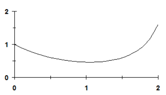
(a) The analytical solution can be derived by separation of variables

$$\begin{array}{rl}& \int \frac{dy}{y}=\int x^2-1.1dx\\ & \ln y=\frac{x^3}{3}-1.1x+C\end{array}$$

Substituting the initial conditions yields $C=0$. Taking the exponential gives the final result

$$y=e^{\frac{x^3}{3}-1.1x}$$

The result can be plotted as

(b) Euler's method with $h=0.5$ gives

$x$	$y$	$\mathrm{d}y/\mathrm{d}x$
0	1	-1.1
0.5	0.45	-0.3825
1	0.25875	-0.02588
1.5	0.245813	0.282684
2	0.387155	1.122749

Euler's method with $h=0.25$ gives

$x$	$y$	$\mathrm{d}y/\mathrm{d}x$
0	1	-1.1
0.25	0.725	-0.75219
0.5	0.536953	-0.45641
0.75	0.422851	-0.22728
1	0.36603	-0.0366
1.25	0.356879	0.165057
1.5	0.398143	0.457865
1.75	0.51261	1.005997
2	0.764109	2.215916

(c) For Heun's method, the value of the slope at $x=0$ can be computed as $-1.1$ which can be used to compute the value of $y$ at the end of the interval as

$$y(0.5)=1+(0-1.1(1))0.5=0.45$$

The slope at the end of the interval can be computed as

$$y^{\prime }(0.5)=0.45(0.5{)}^2-1.1(0.45)=-0.3825$$

which can be averaged with the initial slope to predict

$$y(0.5)=1+\frac{-1.1-0.3825}{2}0.5=0.629375$$

This formula can then be iterated to yield

$j$	$y_i^j$	$\left|{\epsilon }_a\right|$
0	0.45
1	0.629375	$28.5\mathrm{\%}$
2	0.5912578	$6.45\mathrm{\%}$
3	0.5993577	$1.35\mathrm{\%}$
4	0.5976365	$0.288\mathrm{\%}$

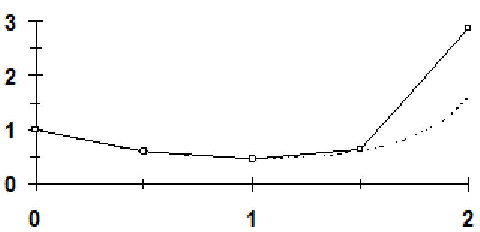
The remaining steps can be implemented with the result

$x_i$	$y_i$
0	1.0000000
0.5	0.5976365
1	0.4590875
1.5	0.6269127
2	2.8784358

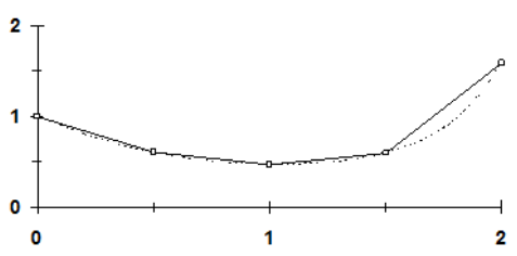
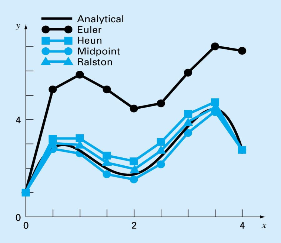
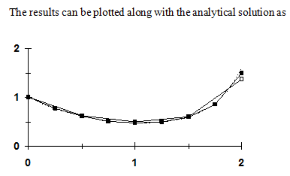
The results along with the analytical solution are displayed below:

(d) The midpoint method with $h=0.5$

$x$	$y$	$\mathrm{d}y/\mathrm{d}x$	$y_m$	$\mathrm{d}y/\mathrm{d}x-\text{mid}$
0	1	-1.1	0.725	-0.75219
0.5	0.623906	-0.53032	0.491326	-0.26409
1	0.491862	-0.04919	0.479566	0.221799
1.5	0.602762	0.693176	0.776056	1.52301
2	1.364267	3.956374	2.35336	9.32519

with $h=0.25$ gives

$x$	$y$	$\mathrm{d}y/\mathrm{d}x$	$y_m$	$\mathrm{d}y/\mathrm{d}x-\text{mid}$
0	1	-1.1	0.8625	-0.93527
0.25	0.766182	-0.79491	0.666817	-0.63973
0.5	0.60625	-0.51531	0.541836	-0.38436
0.75	0.510158	-0.27421	0.475882	-0.15912
1	0.470378	-0.04704	0.464498	0.076932
1.25	0.489611	0.226445	0.517916	0.409478
1.5	0.59198	0.680777	0.677077	1.043122
1.75	0.852761	1.673543	1.061954	2.565282
2	1.494081	4.332836	2.035686	6.953139

(d) The $4^{\text{th }}$-order RK method with $h=0.5$ gives

$x$	$y$	$k_{\mathbf{1}}$	$y_m$	$k_2$	$y_m$	$k_3$	$y_e$	$k_4$	$\varphi$
0	1	-1.1	0.725	-0.75219	0.811953	-0.8424	0.578799	-0.49198	-0.79686
0.5	0.60157	-0.51133	0.473737	-0.25463	0.537912	-0.28913	0.457006	-0.0457	-0.27409
1	0.464524	-0.04645	0.452911	0.209471	0.516892	0.239062	0.584055	0.671663	0.253713
1.5	0.59138	0.680087	0.761402	1.494252	0.964943	1.893701	1.538231	4.460869	1.986144
2	1.584452	4.594911	2.73318	10.83023	4.292008	17.00708	10.08799	51.95317	18.70378