Internal Flows

Introduction

1. Liquid or gas flow through pipes or ducts is commonly used in heating and cooling applications and fluid distribution networks
2. The fluid in such applications is usually forced to flow by a fan or a pump through a flow section.
3. We pay particular attention to friction, which is directly related to pressure drop and head loss during flow through pipes and ducts
4. The pressure drop is then used to determine the pumping power requirement.

Circular pipes can withstand large pressure difference between the inside and outside without undergoing any significant distortion.

However:

1. Theoretical solutions are obtained only for a few simple cases such as fully developed laminar flow in a circular pipe
2. Therefore, we must rely on experimental results and empirical relations for most fluidflow problem rather than closed-form analytical solutions.

The value of the average velocity $V_{\mathrm{avg}}$ at some streamwise cross-section is determined from the requirement that the conservation of mass principle be satisfied:

$$\begin{array}{c}\dot{m}=\rho V_{\mathrm{avg}}{A}_c={\int }_{A_c}\rho u(r)\mathrm{d}{A}_c.\\ V_{\mathrm{avg}}=\frac{{\int }_{A_c}\rho u(r)\mathrm{d}{A}_c}{\rho A_c}=\frac{{\int }_0^R\rho u(r)2\pi r\mathrm{d}r}{\rho \pi R^2}=\frac{2}{R^2}{\int }_0^{R}u(r)r\mathrm{d}r\end{array}$$

Average velocity $V_{\mathrm{avg}}$ is defined as the average speed through a cross section. For fully developed laminar pipe flow, $V_{\mathrm{avg}}$ is half of the maximum velocity:

$$V_{\mathrm{avg}}=\frac{1}{2}{V}_{\max }$$

Laminar and Turbulent Flows

Laminar Flow in Pipes

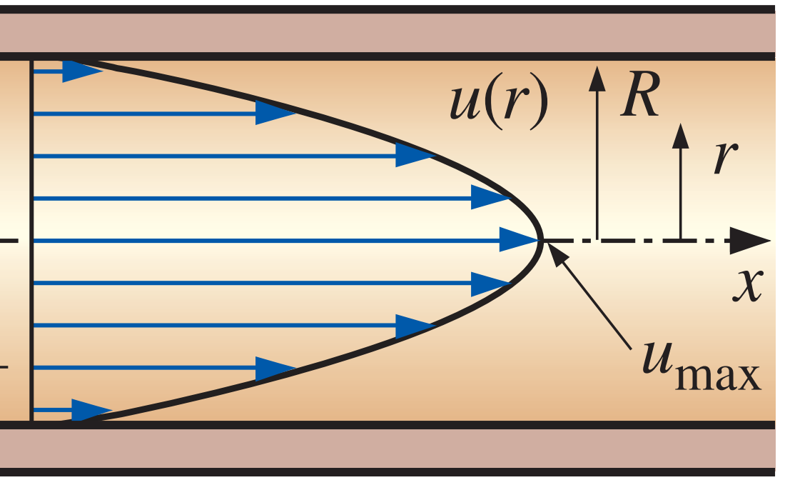
We consider steady, laminar, incompressible flow of a fluid with constant properties in the fully developed region of a straight circular pipe.

In fully developed laminar flow:

• each fluid particle moves at a constant axial velocity along a streamline and the velocity profile $u(r)$ remains unchanged in the flow direction.

$$\begin{array}{c}u(r)=2V_{\mathrm{avg}}(1-\frac{r^2}{R^2})\\ u_{\max }=2V_{\mathrm{avg}}\end{array}$$

• There is no motion in the radial direction, and thus the velocity component in the direction normal to the pipe axis is everywhere zero.
• There is no acceleration since the flow is steady and fully developed.

Laminar and Turbulent Flows

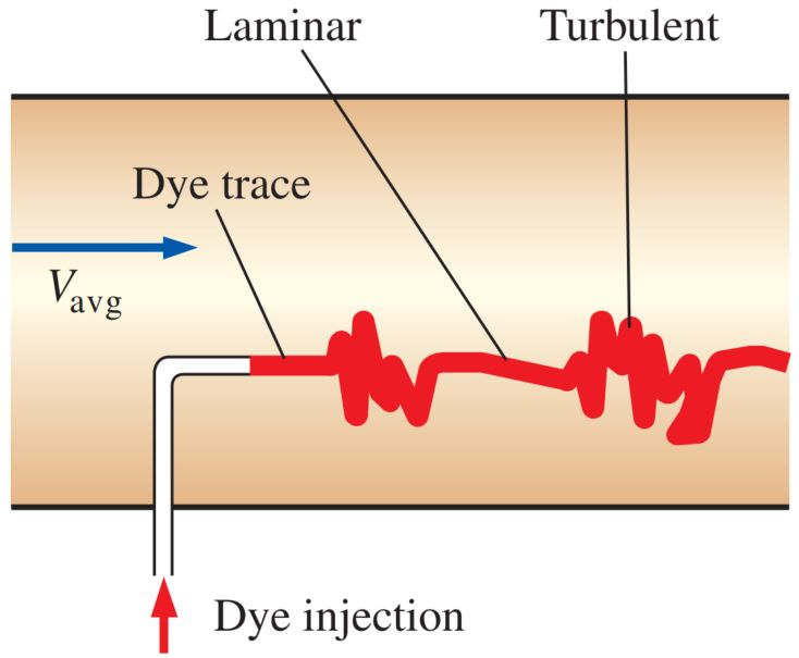
• Laminar: smooth streamlines and highly ordered motion
  • Laminar flow is encountered when highly viscous fluids such as oils flow in small pipes or narrow passages.
• Transition: the flow fluctuates between laminar and turbulent flows.
  • In the transitional flow region, the flow switches between laminar and turbulent seemingly random.
• Turbulent: ...
  • Most flows encountered in practice are turbulent

Reynolds Number

The Reynolds number can be viewed as the ratio of inertial forces to viscous forces acting on a fluid element.

$$\mathrm{Re}=\frac{\mathrm{Internal}\mathrm{Forces}}{\mathrm{Viscous}\mathrm{Forces}}=\frac{V_{\mathrm{avg}}D}{v}=\frac{\rho V_{\mathrm{avg}}D}{\mu }.$$

• At small Reynolds numbers, the viscous forces are large enough to suppress these fluctuations and to keep the fluid ‘in line’ (laminar).
• At large Reynolds numbers, the inertial forces, which are promotional to the fluid density and the fluid velocity, are large relative to viscous forces cannot prevent the viscous forces, and thus the random and rapid fluctuations of the fluid (turbulent).

Critical Reynolds number, ${\mathrm{Re}}_{\mathrm{cr}}$: the Reynolds number at which the flow becomes turbulent

• The value of critical Reynolds number is different for different geometries and flow conditions
• For flow in circular pipe:$$\begin{array}{rlr}& \mathrm{Re}\lesssim 2300& \text{ laminar flow }\\ 2300\lesssim & \mathrm{Re}\lesssim 10,000& \text{ transitional flow }\\ & \mathrm{Re}\gtrsim 10,000& \text{ turbulent flow }\end{array}$$

About the calculation of $D$: For flow through noncircular pipes, the Reynolds number is based on the hydraulic diameter $D_H$ (水力直径):

$$D_H=\frac{4A_c}{p}.$$

where $A_c$ is the cross-sectional area of the flow, $p$ is the perimeter of the cross-section. And for crcular pipes, it reduces to ordinary diameter.

• Circular tube with diameter $D$$$D_H=\frac{4(\pi D^2/4)}{\pi D}=D$$
• Square duct with $a\times a$:$$D_H=\frac{4a^2}{4a}=a$$
• Rectangular duct with $a\times b$:$$D_H=\frac{4ab}{2(a+b)}=\frac{2ab}{a+b}$$
• Channel with width $b$ and height of fluid $a$ (not full, the height of channel is larger than $a$):$$D_H=\frac{4ab}{2a+b}$$

The Entrance Region

• Velocity boundary layer: The region of the flow in which the effects of the viscous shearing forces caused by fluid viscosity are felt.
• Boundary layer region: The viscous effects and the velocity changes are significant.
• Irrotational (core) flow region: The frictional effects are negligible and the velocity remains essentially constant in the radial direction.

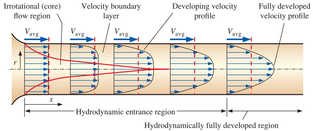
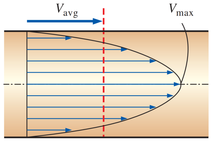
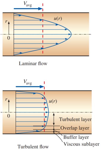
The development of the velocity boundary layer in a pipe. The developed average velocity profile is parabolic in laminar flow, but somewhat flatter or fuller in turbulent flow.

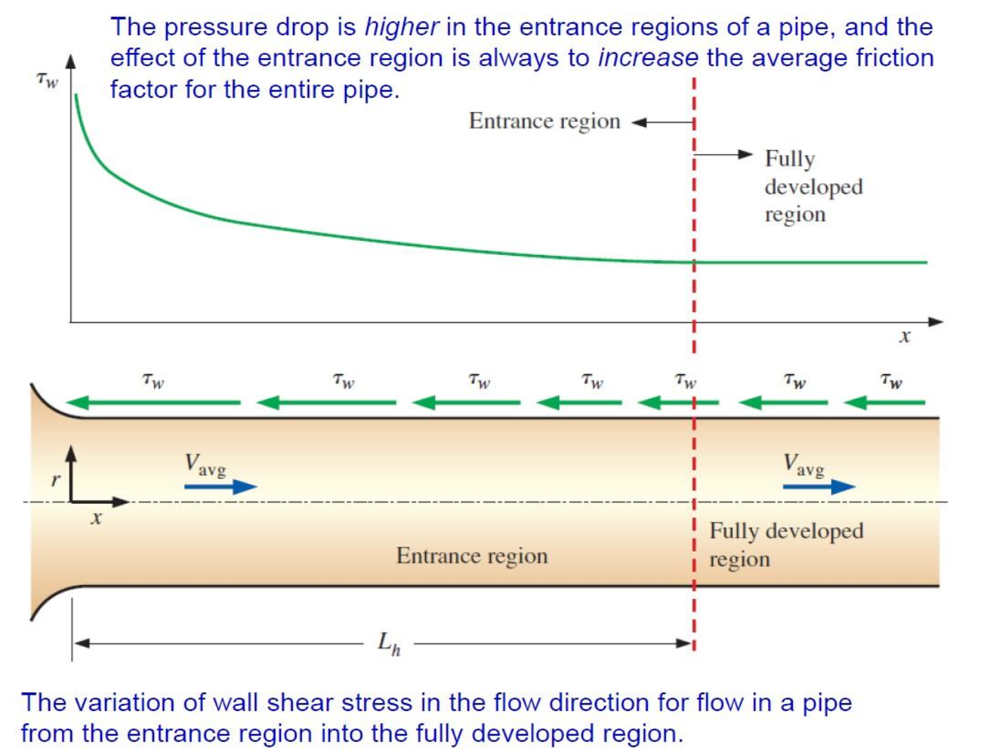
• Hydrodynamic entrance region: The region from the pipe inlet to the point at which the boundary layer merges at the centerline: $V(r,x)$

  • Hydrodynamic entry length $L_h$: The length of this region.
  • Hydrodynamically developing flow: Flow in the entrance region. This is the region where the velocity profile develops.

• Hydrodynamically fully developed region: The region beyond the entrance region in which the velocity profile is fully developed and remains unchanged: $V(r)$

  • Fully developed: When both the velocity profile and the normalized temperature profile remain unchanged.
  $$\frac{\partial u(r,x)}{\partial x}=0⟹u=u(r).$$

  In the fully developed flow region of a pipe, the velocity profile does not change downstream, and thus the wall shear stress ${\tau }_w$ remains constant as well.

Entry Lengths

The hydrodynamic entry length $L_h$ is usually taken to be the distance from the pipe entrance to where the wall shear stress (and thus the friction factor)reaches within about 2 percent of the fully developed value.

1. For laminar flow:

$$\frac{L_{h,\mathrm{laminar}}}{D}\cong 0.05\mathrm{Re}$$

2. For turbulent flow:

$$\frac{L_{h,\mathrm{laminar}}}{D}=1.359{\mathrm{Re}}^{1/4}$$

• The pipes used in practice are usually several times the length of the entrance region, and thus the flow through the pipes is often assumed to be fully developed for the entire length of the pipe
• This simplistic approach gives reasonable results for long pipes but sometimes poor results for short ones since it underpredicts the wall shear stress and thus the friction factor

Quiz: Flow in a pipe is internal flow (T/F?)

True

Quiz: Open-channel flow, flow in a close reactor, flow in a closed valve, which one is NOT internal flow?

Open-channel flow

Quiz: The critical Reynolds number for pipe flow is

2300

Quiz: ${\mathrm{Re}}_D=\frac{\rho u_{m}D}{\mu };{\mathrm{Re}}_D=\frac{u_{m}D}{v},v=\frac{\mu }{\rho };{\mathrm{Re}}_D=\frac{4\dot{m}}{\pi D\mu }$, which are correct for pipe flow

ALL

Laminar Flow in pipes

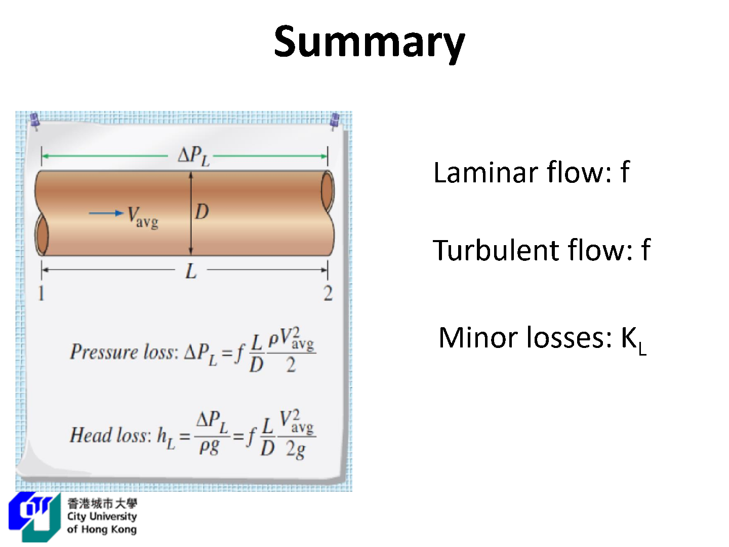
Pressure Drop and Head Loss

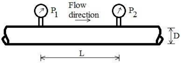
A quantity of interest in the analysis of pipe flow is the pressure drop $\mathrm{\Delta }P$ since it is directly related to the power requirements of the fan or pump to maintain flow. We note that $\mathrm{d}P/\mathrm{d}x=\mathrm{constant}$, and integrating from $x=x_1+L$ where the pressure $P_2$ gives

$$\frac{\mathrm{d}P}{\mathrm{d}x}=\frac{P_2-P_1}{L}$$

For the laminar flow:

$$\mathrm{\Delta }P=P_1-P_2=\frac{8\mu L{V}_{\mathrm{avg}}}{R^2}=\frac{32\mu L{V}_{\mathrm{avg}}}{D^2}.$$

Definition: pressure loss

A pressure drop due to viscous effects represents an irreversible pressure loss, and it is called pressure loss $\mathrm{\Delta }{P}_L$:

$$\mathrm{\Delta }{P}_L=f\frac{L}{D}\frac{\rho V_{\mathrm{avg}}^2}{2}.$$

for all types of fully developed internal flows, where $f$ is the Darcy friction factor:

$$f=\frac{8{\tau }_w}{\rho V_{\mathrm{avg}}^2}.$$

For laminar flow in the circular pipe:

$$f=\frac{64\mu }{\rho D{V}_{\mathrm{avg}}}=\frac{64}{\mathrm{Re}}.$$

In laminar flow, the friction factor is a function of the Reynolds number only and is independent of the roughness of the pipe surface.

Definition: head loss

The head loss represents the additional height that the fluid needs to be raised by a pump in order to overcome the frictional losses in the pipe:

$$h_L=\frac{\mathrm{\Delta }{P}_L}{\rho g}=f\frac{L}{D}\frac{V_{\mathrm{avg}}^2}{2g}.$$

The relation for pressure loss (and head loss)is one of the most general relations in fluid mechanics, and it is valid for laminar or turbulent flows, circular or noncircular pipes, and pipes with smooth or rough surfaces

For horizonal pipe:

$${\dot{W}}_{\mathrm{pump},L}=\dot{V}\mathrm{\Delta }{P}_L=\dot{V}\rho g{h}_L=\dot{m}g{h}_L$$

where:

$$V_{\mathrm{avg}}=\frac{(P_1-P_2)R^2}{8\mu L}=\frac{(P_1-P_2)D^2}{32\mu L}=\frac{\mathrm{\Delta }P{D}^2}{32\mu L}$$

and the volume flow rate $\dot{V}$ (Poiseuill's Law):

$$\dot{V}=V_{\mathrm{avg}}{A}_c=\frac{(P_1-P_2)R^2}{8\mu L}\pi R^2=\frac{(P_1-P_2)\pi D^4}{128\mu L}=\frac{\mathrm{\Delta }P\pi D^4}{128\mu L}.$$

The pumping power requirement for a laminar flow piping system can be reduced by a factor of $16$ by doubling the pipe diameter.

The pressure drop $\mathrm{\Delta }P$ equals the pressure loss $\mathrm{\Delta }{P}_L$ in the case of a horizontal pipe, but this is not the case for inclined pipes or pipes with variable cross-sectional area

This can be demonstrated by writing the energy equation for steady, imcompressible one-dimensional flow in terms of heads as

$$\begin{array}{c}\frac{P_1}{\rho g}+{\alpha }_1\frac{V_1^2}{2g}+z_1+h_{\mathrm{pump},u}=\frac{P_2}{\rho g}+{\alpha }_2\frac{V_2^2}{2g}+z_2+h_{\mathrm{turbine},e}+h_L\\ P_1-P_2=\rho ({\alpha }_2{V}_2^2-{\alpha }_1{V}_1^2)/2+\rho g[(z_2-z_1)+h_{\mathrm{turbine},e}-h_{\mathrm{pump},u}+h_L]\end{array}$$

A useful equation to calculate the pressure drop for horizontal pipes and non-horizontal pipes

Laminar Flow in Noncircular Pipes

The friction factor f relations are given in Table below for fully developed laminar flow in pipes of various cross sections.

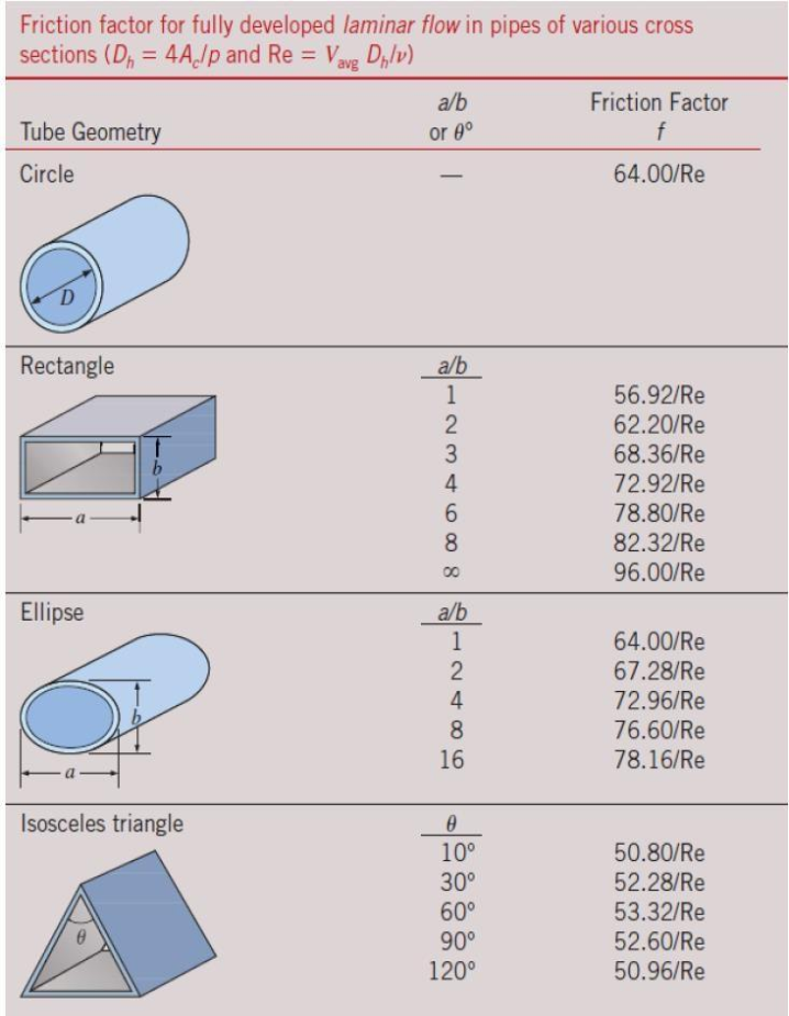
The Reynolds number for flow in these pipes is based on the hydraulic diameter $D_H=4A_c/p$, where $A_c$ is the crosssectional area of the pipe and $p$ is its wetted perimeter

Quiz: For the fully developed laminar flow, we have

$$f=\frac{32}{\mathrm{Re}}$$

Quiz: A pressure drop due to () represents an irreversible pressure loss, and it is called pressure loss.

viscous effect

Examples1: Laminar Flow in Horizonal Pipes

Consider the fully developed flow of glycerin at ${40}^{\circ }\mathrm{C}$ through a $70-\mathrm{m}$-long, $4-\mathrm{cm}$-diameter, horizontal, circular pipe. If the flow velocity at the centerline is measured to be $6\mathrm{m}/\mathrm{s}$, determine the velocity profile and the pressure difference across this $70-\mathrm{m}$-long section of the pipe, and the useful pumping power required to maintain this flow.

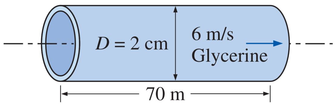
Properties: The density and dynamic viscosity of glycerin at ${40}^{\circ }\mathrm{C}$ are $\rho =1252\mathrm{kg}/{\mathrm{m}}^3$ and $\mu =0.3073\mathrm{kg}/\mathrm{m}\cdot \mathrm{s}$, respectively.

Analysis: The velocity profile in fully developed laminar flow in a circular pipe is expressed as

$$u(r)=u_{max}(1-\frac{r^2}{R^2})$$

Substituting, the velocity profile is determined to be

$$u(r)=(6\mathrm{m}/\mathrm{s})(1-\frac{r^2}{(0.02\mathrm{m}{)}^2})=6(1-2500r^2)$$

where $u$ is in $\mathrm{m}/\mathrm{s}$ and $r$ is in m . The average velocity, the flow rate, and the Reynolds number are

$$\begin{array}{rl}V& =V_{\text{avg }}=\frac{u_{max}}{2}=\frac{6\mathrm{m}/\mathrm{s}}{2}=3\mathrm{m}/\mathrm{s}\\ \dot{V}& =V_{\text{avg }}{A}_c=V\left(\pi D^2/4\right)=(3\mathrm{m}/\mathrm{s})[\pi (0.04\mathrm{m}{)}^2/4]=3.77\times {10}^{-3}{\mathrm{m}}^3/\mathrm{s}\\ \mathrm{Re}& =\frac{\rho VD}{\mu }=\frac{\left(1252\mathrm{kg}/{\mathrm{m}}^3\right)(3\mathrm{m}/\mathrm{s})(0.04\mathrm{m})}{0.3073\mathrm{kg}/\mathrm{m}\cdot \mathrm{s}}=488.9\end{array}$$

which is less than 2300 . Therefore, the flow is indeed laminar. Then the friction factor and the head loss become

$$\begin{array}{rl}f& =\frac{64}{\mathrm{Re}}=\frac{64}{488.9}=0.1309\\ h_L& =f\frac{L{V}^2}{D2g}=0.1309\frac{(70\mathrm{m})}{(0.04\mathrm{m})}\frac{(3\mathrm{m}/\mathrm{s}{)}^2}{2\left(9.81\mathrm{m}/{\mathrm{s}}^2\right)}=105.1\mathrm{m}\end{array}$$

The energy balance for steady, incompressible one-dimensional flow is given by Eq. 8-28 as

$$\frac{P_1}{\rho g}+{\alpha }_1\frac{V_1^2}{2g}+z_1+h_{\text{pump, u }}=\frac{P_2}{\rho g}+{\alpha }_2\frac{V_2^2}{2g}+z_2+h_{\text{turbine, e }}+h_L$$

For fully developed flow in a constant diameter pipe with no pumps or turbines，it reduces to

$$\mathrm{\Delta }P=P_1-P_2=\rho g(z_2-z_1+h_L)$$

Then the pressure difference and the required useful pumping power for the horizontal case become

$$\begin{array}{rl}\mathrm{\Delta }P& =\rho g(z_2-z_1+h_L)\text{ Or }(\mathrm{\Delta }P=\rho g{h}_L)\text{ for horizontal pipe }\\ & =\left(1252\mathrm{kg}/{\mathrm{m}}^3\right)\left(9.81\mathrm{m}/{\mathrm{s}}^2\right)(0+105.1\mathrm{m})\left(\frac{1\mathrm{kPa}}{1000\mathrm{kg}/\mathrm{m}\cdot {\mathrm{s}}^2}\right)\\ & =1291\mathrm{kPa}\\ {\dot{W}}_{\text{pump, u }}& =\dot{V}\mathrm{\Delta }P=(3.77\times {10}^3{\mathrm{m}}^3/\mathrm{s})(1291\mathrm{kPa})\left(\frac{1\mathrm{kW}}{\mathrm{kPa}\cdot {\mathrm{m}}^3/\mathrm{s}}\right)=4.87\mathrm{kW}\end{array}$$

Example2: Pressure Drop and Head Loss in a Pipe

Water at $5^{\circ }\mathrm{C}(\rho =1000\mathrm{kg}/{\mathrm{m}}^3$ and $\mu =1.519\times {10}^{-3}\mathrm{kg}/\mathrm{m}\cdot \mathrm{s})$ is flowing steadily through a $0.3-\mathrm{cm}$ diameter $9-\mathrm{m}$-long horizontal pipe at an average velocity of $0.9\mathrm{m}/\mathrm{s}$ (Fig. 8-18). Determine (a) the head loss, (b) the pressure drop, and (c) the pumping power requirement to overcome this pressure drop.

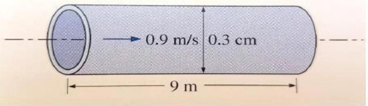
Properties: The density and dynamic viscosity of water are given to be $\rho =1000\mathrm{kg}/{\mathrm{m}}^3$ and $\mu =1.519\times {10}^{-3}\mathrm{kg}/\mathrm{m}\cdot \mathrm{s}$, respectively.

Analysis:

1. First we need to determine the flow regime. The Reynolds number is

$$\mathrm{Re}=\frac{\rho V_{\mathrm{avg}}D}{\mu }=\frac{\left(1000\mathrm{kg}/{\mathrm{m}}^3\right)(0.9\mathrm{m}/\mathrm{s})(0.003\mathrm{m})}{1.519\times {10}^{-3}\mathrm{kg}/\mathrm{m}\cdot \mathrm{s}}=1777$$

which is less than 2300 . Therefore, the flow is laminar. Then the friction factor and the head loss become

$$\begin{array}{rl}f& =\frac{64}{\mathrm{Re}}=\frac{64}{1777}=0.0360\\ h_L& =f\frac{L}{D}\frac{V_{\text{avg }}^2}{2g}=0.0360\frac{9\mathrm{m}}{0.003\mathrm{m}}\frac{(0.9\mathrm{m}/\mathrm{s}{)}^2}{2\left(9.81\mathrm{m}/{\mathrm{s}}^2\right)}=4.46\mathrm{m}\end{array}$$

2. Noting that the pipe is horizontal and its diameter is constant, the pressure drop in the pipe is due entirely to the frictional losses and is equivalent to the pressure loss,

$$\begin{array}{rl}\mathrm{\Delta }P& =\mathrm{\Delta }{P}_L=f\frac{L}{D}\frac{\rho V_{\text{avg }}^2}{2}=0.0360\frac{9\mathrm{m}}{0.003\mathrm{m}}\frac{\left(1000\mathrm{kg}/{\mathrm{m}}^3\right)(0.9\mathrm{m}/\mathrm{s}{)}^2}{2}\left(\frac{1\mathrm{N}}{1\mathrm{kg}\cdot \mathrm{m}/{\mathrm{s}}^2}\right)\\ & =43,740\mathrm{N}/{\mathrm{m}}^2=43.7\mathrm{kPa}\end{array}$$

3. The volume flow rate and the pumping power requirements are

$$\begin{array}{rl}\dot{V}& =V_{\text{avg }}{A}_c=V_{\text{avg }}\left(\pi D^2/4\right)=(0.9\mathrm{m}/\mathrm{s})[\pi (0.003\mathrm{m}{)}^2/4]=6.36\times {10}^{-6}{\mathrm{m}}^3/\mathrm{s}\\ {\dot{W}}_{\text{pump }}& =\dot{V}\mathrm{\Delta }\mathrm{P}=(6.36\times {10}^{-6}{\mathrm{m}}^3/\mathrm{s})(43,740\mathrm{N}/{\mathrm{m}}^2)\left(\frac{1\mathrm{W}}{1\mathrm{N}\cdot \mathrm{m}/\mathrm{s}}\right)=\mathbf{0}\mathbf{.}\mathbf{2}\mathbf{8}\mathbf{W}\end{array}$$

Therefore, power input in the amount of 0.28 W is needed to overcome the frictional losses in the flow due to viscosity.

Discussion: The pressure rise provided by a pump is often listed by a pump manufacturer in units of head (Chap. 14). Thus, the pump in this flow needs to provide 4.46 m of water head in order to overcome the irreversible head loss.

Turbulent Flow in Pipes

Most flows encountered in engineering practice are turbulent, and thus it is important to understand how turbulence affects wall shear stress.

Turbulent flow is a complex mechanism dominated by fluctuations, and it is still not fully understood.

We must rely on experiments and the empirical or semi-empirical correlations developed for various situations.

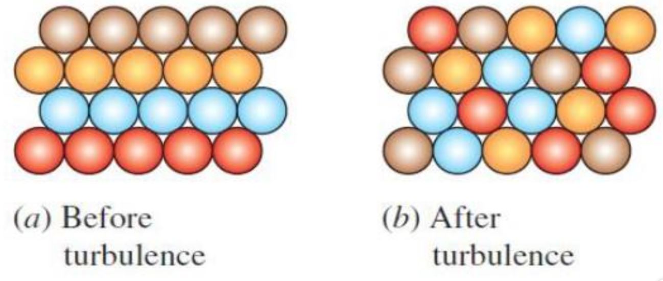
The intense mixing in turbulent flow brings fluid particles at different momentums into close contact and thus enhances momentum transfer.

Turbulent flow is characterized by disorderly and rapid fluctuations of swirling regions of fluid, called eddies, throughout the flow.

These fluctuations provide an additional mechanism for momentum and energy transfer.

In turbulent flow, the swirling eddies transport mass, momentum, and energy to other regions of flow much more rapidly than molecular diffusion, greatly enhancing mass, momentum, and heat transfer.

As a result, turbulent flow is associated with much higher values of friction, heat transfer, and mass transfer coefficients

Turbulent Velocity Profile

• viscous sublayer: The very thin layer next to the wall where viscous effects are dominant is the viscous (or laminar or linear or wall) sublayer
  • The velocity profile in this layer is very nearly linear
• buffer layer: Next to the viscous sublayer is the buffer layer, in which turbulent effects are becoming significant, but the flow is still dominated by viscous effects
• overlap layer: Above the buffer layer is the overlap (or transition) layer, also called the inertial sublayer, in which the turbulent effects are much more significant, but still not dominant
• turbulent layer: Above that is the outer (or turbulent) layer in the remaining part of the flow in which turbulent effects dominate over molecular diffusion (viscous) effects

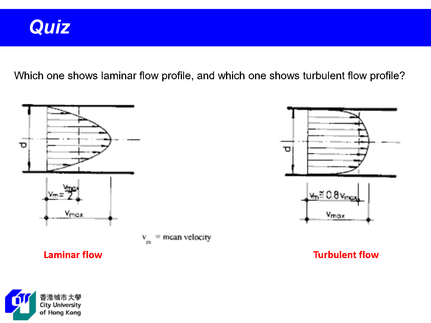
The velocity profile in fully developed pipe flow is parabolic in laminar flow, but much fuller in turbulent flow. Note that $u(r)$ in the turbulent case is the time-averaged velocity component in the axial direction (the overbar on $u$ has been dropped for simplicity).

quiz:

The Moody Chart and the Colebrook Equation

Colebrook Equation (turbulent flow for smooth and rough pipes):

$$\frac{1}{\sqrt{f}}=-2.0\log (\frac{\epsilon /D}{3.7}+\frac{2.51}{\mathrm{Re}\sqrt{f}})$$

• The friction factor in fully developed turbulent pipe flow depends on the Reynolds number and the relative roughness $\epsilon /D$.
• The friction factor is minimum for a smooth pipe $(\epsilon /D=0)$ and increases with roughness
• The Colebrook equation is implicit in $f$ since $f$ appears on both sides of the equation. It must be solved iteratively.

Here is the Moody Chart. It presents the Darcy friction factor for pipe flow as a function of Reynolds number and $\epsilon /D$ over a wide range.

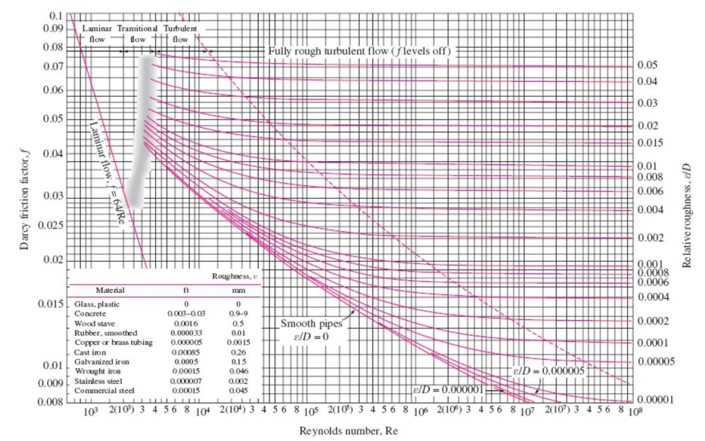
Quiz: In the ‘Fully Rough Zone’ for a given relative roughness, the friction factor is:

A constant

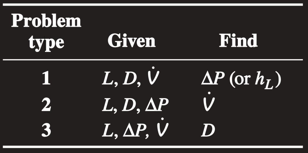
Types of Fluid Flow Problems

1. Determining the pressure drop (or head loss) when the pipe length and diameter are given for a specified flow rate (or velocity)
2. Determining the flow rate when the pipe length and diameter are given for a specified pressure drop (or head loss)
3. Determining the pipe diameter when the pipe length and flow rate are given for a specified pressure drop (or head loss)

To avoid tedious iterations in head loss, flow rate, and diameter calculations, these explicit relations (Swamee-Jain formula) that are accurate to within 2 percent of the Moody chart may be used:

$$\begin{array}{rl}& h_L=1.07\frac{{\dot{V}}^{2}L}{g{D}^5}{\{\ln [\frac{\epsilon }{3.7D}+4.62{\left(\frac{\nu D}{\dot{V}}\right)}^{0.9}]\}}^{-2}{10}^{-6}<\epsilon /D<{10}^{-2}3000<\mathrm{Re}<3\times {10}^8\\ & \dot{V}=-0.965{\left(\frac{g{D}^5{h}_L}{L}\right)}^{0.5}\ln [\frac{\epsilon }{3.7D}+{\left(\frac{3.17v^{2}L}{g{D}^3{h}_L}\right)}^{0.5}]\mathrm{Re}>2000\\ & D=0.66{[{\epsilon }^{1.25}{\left(\frac{L{\dot{V}}^2}{g{h}_L}\right)}^{4.75}+\nu {\dot{V}}^{9.4}{\left(\frac{L}{g{h}_L}\right)}^{5.2}]}^{0.04}{10}^{-6}<\epsilon /D<{10}^{-2}5000<\mathrm{Re}<3\times {10}^8\end{array}$$

Example3: Determining the Head Loss in a Water Pipe

Water at ${15}^{\circ }\mathrm{C}(\rho =999\mathrm{kg}/{\mathrm{m}}^3$ and $\mu =1.138\times {10}^{-3}\mathrm{kg}/\mathrm{m}\cdot \mathrm{s})$ is flowing steadily in a 5 -cm-diameter horizontal pipe made of stainless steel at a rate of $6\mathrm{L}/\mathrm{s}$ (Fig. 8-32). Determine the pressure drop, the head loss, and the required pumping power input for flow over a $60-\mathrm{m}$-long section of the pipe.

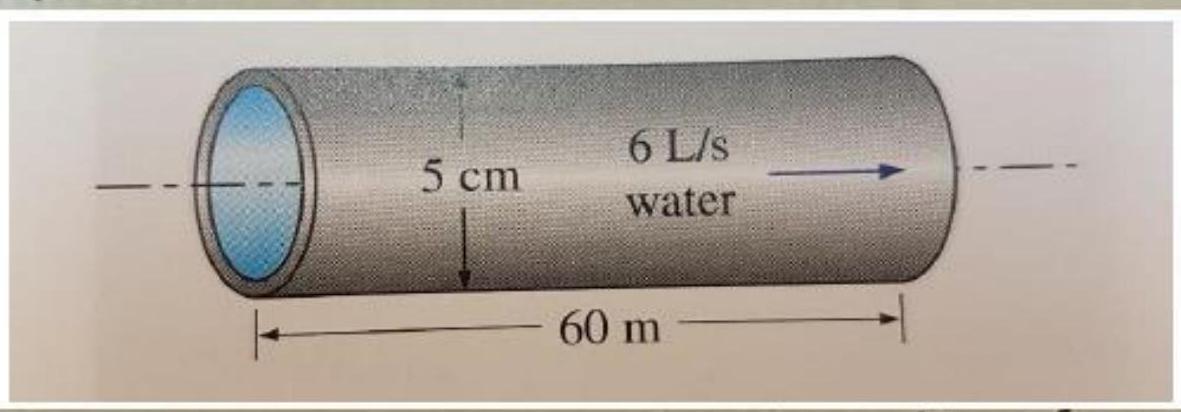
Properties: The density and dynamic viscosity of water are given $999\mathrm{kg}/{\mathrm{m}}^3$ and $\mu =1.138\times {10}^{-3}\mathrm{kg}/\mathrm{m}\cdot \mathrm{s}$, respectively.

Analysis: We recognize this as a problem of the first type, since flow rate, pipe length, and pipe diameter are known. First we calculate the average velocity and the Reynolds number to determine the flow regime:

$$\begin{array}{rl}V& =\frac{\dot{V}}{A_c}=\frac{\dot{V}}{\pi D^2/4}=\frac{0.006{\mathrm{m}}^3}{\pi (0.05\mathrm{m}{)}^2/4}=3.06\mathrm{m}/\mathrm{s}\\ \mathrm{Re}& =\frac{\rho VD}{\mu }=\frac{\left(999\mathrm{kg}/{\mathrm{m}}^3\right)(3.06\mathrm{m}/\mathrm{s})(0.05\mathrm{m})}{1.138\times {10}^{-3}\mathrm{kg}/\mathrm{m}\cdot \mathrm{s}}=134,300\end{array}$$

Since $\mathrm{Re}$ is greater than $4000$, the flow is turbulent. The relative roughness of the pipe is estimated using Table 8-2

$$\epsilon /D=\frac{0.002\mathrm{mm}}{50\mathrm{mm}}=0.000040$$

The friction factor corresponding to this relative roughness and Reynolds number is determined from the Moody chart. To avoid any reading error, we determine $f$ from the Colebrook equation on which the Moody chart is based:

$$\begin{array}{rl}& \frac{1}{\sqrt{f}}=-2.0\log (\frac{\epsilon /D}{3.7}+\frac{2.51}{\mathrm{Re}\sqrt{f}})\\ \to & \frac{1}{\sqrt{f}}=-2.0\log (\frac{0.000040}{3.7}+\frac{2.51}{134,300\sqrt{f}}).\end{array}$$

Using an equation solver or an iterative scheme, the friction factor is determined to be $f=0.0172$. Then the pressure drop (which is equivalent to pressure loss in this case), head loss, and the required power input become

$$\begin{array}{r}\begin{array}{rl}\mathrm{\Delta }P=\mathrm{\Delta }{P}_L=f\frac{L}{D}\frac{\rho V^2}{2}& =0.0172\frac{60\mathrm{m}}{0.05\mathrm{m}}\frac{\left(999\mathrm{kg}/{\mathrm{m}}^3\right)(3.06\mathrm{m}/\mathrm{s}{)}^2}{2}\left(\frac{1\mathrm{N}}{1\mathrm{kg}\cdot \mathrm{m}/{\mathrm{s}}^2}\right)\\ & =96,540\mathrm{N}/{\mathrm{m}}^2=96.5\mathrm{kPa}\\ h_L=\frac{\mathrm{\Delta }{P}_L}{\rho g}=f\frac{L}{D}\frac{V^2}{2g}& =0.0172\frac{60\mathrm{m}}{0.05\mathrm{m}}\frac{(3.06\mathrm{m}/\mathrm{s}{)}^2}{2\left(9.81\mathrm{m}/{\mathrm{s}}^2\right)}=9.85\mathrm{m}\\ {\dot{W}}_{\text{pump }}=\dot{V}\mathrm{\Delta }P& =\left(0.006{\mathrm{m}}^3/\mathrm{s}\right)(96,540\mathrm{N}/{\mathrm{m}}^2)\left(\frac{1\mathrm{W}}{1\mathrm{N}\cdot \mathrm{m}/\mathrm{s}}\right)=579\mathrm{W}\end{array}\end{array}$$

Therefore, power input in the amount of $579\mathrm{W}$ is needed to overcome the frictional losses in the pipe.

Discussion: It is common practice to write our final answers to three signififrictional digits, even though we know that the results are accurate to at most two significant digits because of inherent inaccuracies in the Colebrook equation, as discussed previously.

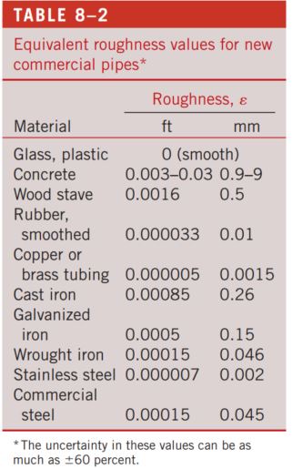
Example4: Determining the Diameter of an Air Duct [core]

Heated air at 1 atm and ${35}^{\circ }\mathrm{C}$ is to be transported in a $150-\mathrm{m}$-long circular plastic duct at a rate of $0.35{\mathrm{m}}^3/\mathrm{s}$ (Fig. 8-33). If the head loss in the pipe is not to exceed 20 m , determine the minimum diameter of the duct.

Properties: The density, dynamic viscosity, and kinematic viscosity of air at ${35}^{\circ }\mathrm{C}$ are $\rho =1.145\mathrm{kg}/{\mathrm{m}}^3,\mu =1.895\times {10}^{-5}\mathrm{kg}/\mathrm{m}\cdot \mathrm{s}$, and $\nu =1.655\times {10}^{-5}{\mathrm{m}}^2/\mathrm{s}$.

Analysis: This is a problem of the third type since it involves the determination of diameter for specified flow rate and head loss. We can solve this problem using three different approaches:

1. an iterative approach by assuming a pipe diameter, calculating the head loss, comparing the result to the specified head loss, and repeating calculations until the calculated head loss matches the specified value;
2. writing all the relevant equations (leaving the diameter as an unknown) and solving them simultaneously using an equation solver; and
3. using the third Swamee-Jain formula. We will demonstrate the use of the last two approaches.

The average velocity, the Reynolds number, the friction factor, and the head loss relations are expressed as ( $D$ is in $\mathrm{m},V$ is in $\mathrm{m}/\mathrm{s}$, and $\mathrm{Re}$ and $f$ are dimensionless)

$$\begin{array}{rl}\mathrm{Re}& =\frac{VD}{\nu }=\frac{VD}{1.655\times {10}^{-5}{\mathrm{m}}^2/\mathrm{s}}\\ \frac{1}{\sqrt{f}}& =-2.0\log (\frac{\epsilon /D}{3.7}+\frac{2.51}{\mathrm{Re}\sqrt{f}})=-2.0\log \left(\frac{2.51}{\mathrm{Re}\sqrt{f}}\right)\\ h_L& =f\frac{L}{D}\frac{V^2}{2g}\to 20\mathrm{m}=f\frac{150\mathrm{m}}{D}\frac{V^2}{2\left(9.81\mathrm{m}/{\mathrm{s}}^2\right)}\end{array}$$

The roughness is approximately zero for a plastic pipe (Table 8-2). Therefore, this is a set of four equations and four unknowns, and solving them with an equation solver such as EES gives

$$D=0.267\mathrm{m},f=0.0180,V=6.24\mathrm{m}/\mathrm{s},\text{ and }\mathrm{Re}=100,800$$

Therefore, the diameter of the duct should be more than $26.7\mathrm{cm}$ if the head loss is not to exceed $20\mathrm{m}$ . Note that $\mathrm{Re}>4000$, and thus the turbulent flow assumption is verified.

The diameter can also be determined directly from the third Swamee-Jain formula to be

$$\begin{array}{rl}D& =0.66{[{\epsilon }^{1.25}{\left(\frac{L{\dot{V}}^2}{g{h}_L}\right)}^{4.75}+\nu {\dot{V}}^{9.4}{\left(\frac{L}{g{h}_L}\right)}^{5.2}]}^{0.04}\\ & =0.66{[0+(1.655\times {10}^{-5}{\mathrm{m}}^2/\mathrm{s}){\left(0.35{\mathrm{m}}^3/\mathrm{s}\right)}^{9.4}{\left(\frac{150\mathrm{m}}{\left(9.81\mathrm{m}/{\mathrm{s}}^2\right)(20\mathrm{m})}\right)}^{5.2}]}^{0.04}\\ & =0.271\mathrm{m}\end{array}$$

Example5: Determining the Flow Rate of Air in a Duct

Reconsider Example4. Now the duct length is doubled while its diameter is maintained constant. If the total head loss is to remain constant, determine the drop in the flow rate through the duct.

SOLUTION: The diameter and the head loss in an air duct are given. The drop in the flow rate is to be determined.

Analysis: This is a problem of the second type since it involves the determination of the flow rate for a specified pipe diameter and head loss. The solution involves an iterative approach since the flow rate (and thus the flow velocity) is not known.

The average velocity, Reynolds number, friction factor, and the head loss relations are expressed as ( $D$ is in $\mathrm{m},V$ is in $\mathrm{m}/\mathrm{s}$, and $\mathrm{Re}$ and $f$ are dimensionless)

The average velocity, Reynolds number, friction factor, and the head loss relations are expressed as ( $D$ is in $\mathrm{m},V$ is in $\mathrm{m}/\mathrm{s}$, and $\mathrm{Re}$ and $f$ are dimensionless)

$$\begin{array}{rl}V& =\frac{\dot{V}}{A_c}=\frac{\dot{V}}{\pi D^2/4}\to V=\frac{\dot{V}}{\pi (0.267\mathrm{m}{)}^2/4}\\ \mathrm{Re}& =\frac{VD}{\nu }\to \mathrm{Re}=\frac{V(0.267\mathrm{m})}{1.655\times {10}^{-5}{\mathrm{m}}^2/\mathrm{s}}\\ \frac{1}{\sqrt{f}}& =-2.0\log (\frac{\epsilon /D}{3.7}+\frac{2.51}{\mathrm{Re}\sqrt{f}})\to \frac{1}{\sqrt{f}}=-2.0\log \left(\frac{2.51}{\mathrm{Re}\sqrt{f}}\right)\\ h_L& =f\frac{L}{D}\frac{V^2}{2g}\to 20\mathrm{m}=f\frac{300\mathrm{m}}{0.267\mathrm{m}}\frac{V^2}{2\left(9.81\mathrm{m}/{\mathrm{s}}^2\right)}\end{array}$$

This is a set of four equations in four unknowns and solving them with an equation solver such as EES gives

$$\dot{V}=0.24{\mathrm{m}}^3/\mathrm{s},f=0.0195,V=4.23\mathrm{m}/\mathrm{s},\text{ and }\mathrm{Re}=68,300$$

Then the drop in the flow rate becomes

$${\dot{V}}_{\text{drop }}={\dot{V}}_{\text{old }}-{\dot{V}}_{\text{new }}=0.35-0.24=\mathbf{0}\mathbf{.}\mathbf{1}\mathbf{1}{\mathrm{m}}^3/\mathrm{s}(\text{ a drop of }31\text{ percent })$$

Therefore, for a specified head loss (or available head or fan pumping power), the flow rate drops by about $31$ percent from $0.35$ to $0.24{\mathrm{m}}^3/\mathrm{s}$ when the duct length doubles.

Minor Losses

The fluid in a typical piping system passes through various fittings, valves, bends, elbows, tees, inlets, exits, enlargements, and contractions in addition to the pipes.

These components interrupt the smooth flow of the fluid and cause additional losses because of the flow separation and mixing they induce.

minor losses

In a typical system with long pipes, these losses are minor compared to the head loss in the straight sections (the major losses) and are called minor losses

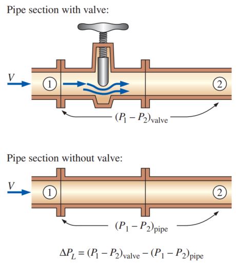
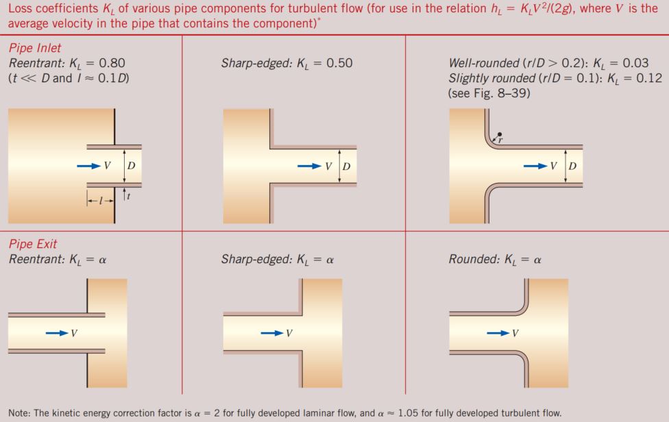
For a constant-diameter section of a pipe with a minor loss component, the loss coefficient of the component (such as the gate valve shown) is determined by measuring the additional pressure loss it causes and dividing it by the dynamic pressure in the pipe.

Minor losses are usually expressed in terms of the loss coefficient $K_L$:

$$K_L=\frac{h_L}{V^2/(2g)}.$$

where $h_L$ is head loss due to component, and is defined as $h_L=\mathrm{\Delta }{P}_L/\rho g$.

When the inlet diameter equals the outlet diameter, the loss coefficient of a component can also be determined by measuring the pressure loss across the component and dividing it by the dynamic pressure

$$K_L=\mathrm{\Delta }{P}_L/(\rho V^2/2)$$

When the loss coefficient for a component is available, the head loss for that component is determined from minor loss:

$$h_L=K_L\frac{V^2}{2g}$$

Minor losses are also expressed in terms of the equivalent length $L_{\mathrm{equiv}}$:

$$h_L=K_L\frac{V^2}{2g}=f\frac{L_{\mathrm{equiv}}}{D}\frac{V^2}{2g}⟹L_{\mathrm{equiv}}=\frac{D}{f}{K}_L$$

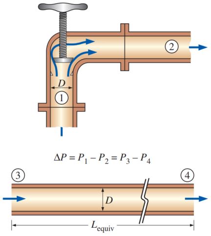
The head loss caused by a component (such as the angle valve shown) is equivalent to the head loss caused by a section of the pipe whose length is the equivalent length.

Total head Losses

Once the loss coefficients are available, the total head loss in a piping system is determined from:

$$\begin{array}{rlrl}{h}_{L,\mathrm{total}}& =h_{L,\mathrm{major}}& & +h_{L,\mathrm{minor}}\\ & =\sum _i{f}_i\frac{L_i}{D_i}\frac{V_i^2}{2g}& & +\sum _j{K}_{L,j}\frac{V_i^2}{2g}\end{array}$$

Example for Minor Losses

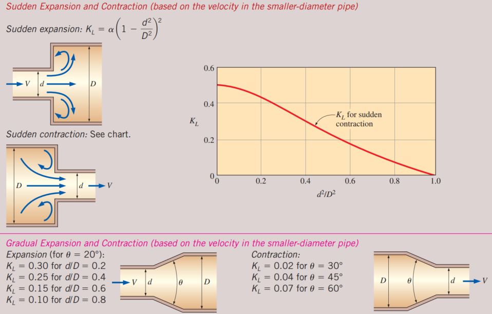
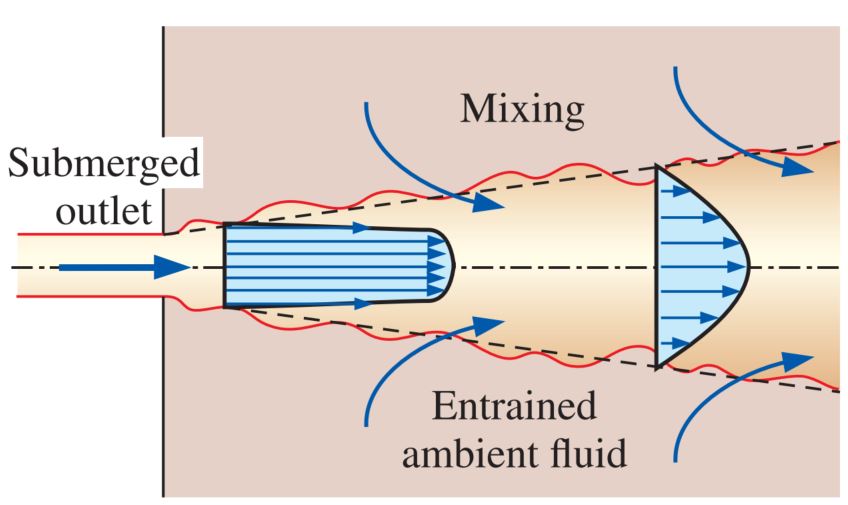
Sudden Expansion: All the kinetic energy of the flow is “lost” (turned into thermal energy) through friction as the jet decelerates and mixes with ambient fluid downstream of a submerged outlet.

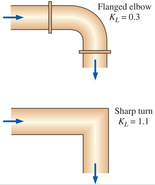
The losses during changes of direction can be minimized by making the turn “easy” on the fluid by using circular arcs instead of sharp turns.

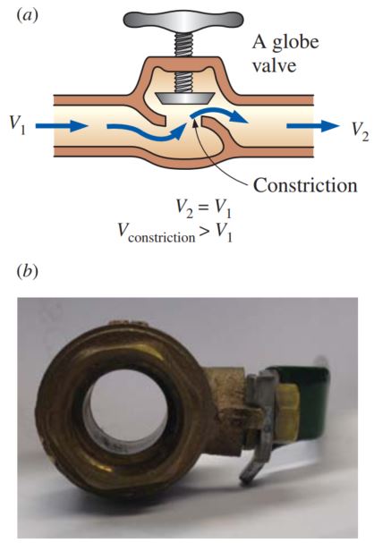
(a) The large head loss in a partially closed globe valve is due to irreversible deceleration, flow separation, and mixing of highvelocity fluid coming from the narrow valve passage.

(b) The head loss through a fully-open ball valve, on the other hand, is quite small. (Photo by John M. Cimbala)

Quiz: Major losses are greater than minor losses (T/F?)

False

Quiz: Slight rounding of the edge can result in a significant reduction of loss coefficient (T/F?)

True

Example6: Head Loss and Pressure Rise during Gradual Expansion

A 6-cm-diameter horizontal water pipe expands gradually to a 9-cm-diameter pipe (Fig. 8-43). The walls of the expansion section are angled ${10}^{\circ }$ from the axis. The average velocity and pressure of water before the expansion section are $7\mathrm{m}/\mathrm{s}$ and $150\mathrm{kPa}$ , respectively. Determine the head loss in the expansion section and the pressure in the larger-diameter pipe.

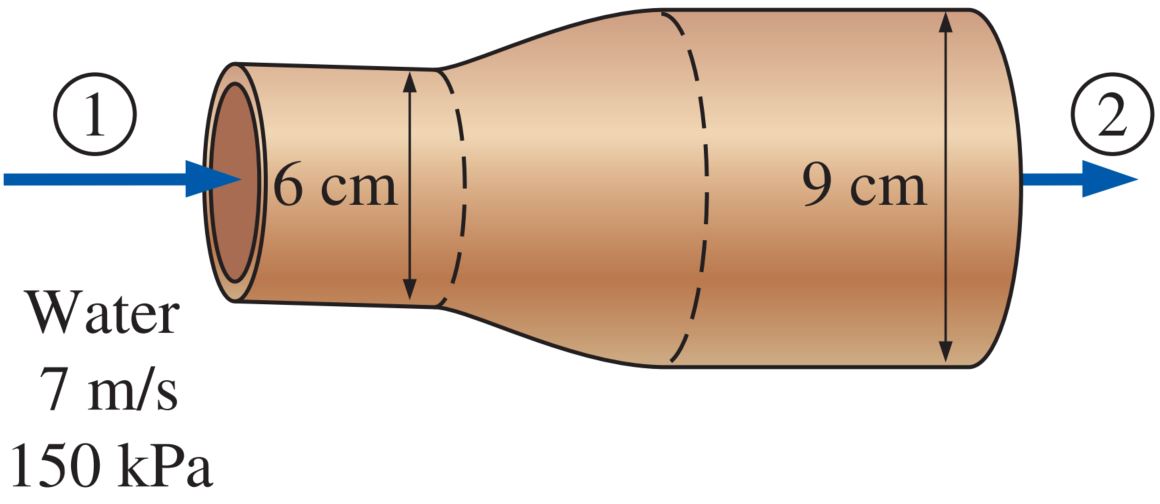
Assumptions

1. The flow is steady and incompressible.
2. The flow at sections 1 and 2 is fully developed and turbulent with ${\alpha }_1={\alpha }_2\cong 1.06$.

Properties: We take the density of water to be $\rho =1000\mathrm{kg}/{\mathrm{m}}^3$. The loss coefficient for a gradual expansion of total included angle $\theta ={20}^{\circ }$ and diameter ratio $d/D=6/9$ is $K_L=0.133$ (by interpolation using Table 8-4).

Analysis: Noting that the density of water remains constant, the downstream velocity of water is determined from conservation of mass to be

$$\begin{array}{rl}{\dot{m}}_1={\dot{m}}_2\to \rho V_1{A}_1& =\rho V_2{A}_2\to V_2=\frac{A_1}{A_2}{V}_1=\frac{D_1^2}{D_2^2}{V}_1\\ V_2& =\frac{(0.06\mathrm{m}{)}^2}{(0.09\mathrm{m}{)}^2}(7\mathrm{m}/\mathrm{s})=3.11\mathrm{m}/\mathrm{s}\end{array}$$

Then the irreversible head loss in the expansion section becomes

$$h_L=K_L\frac{V_1^2}{2g}=(0.133)\frac{(7\mathrm{m}/\mathrm{s}{)}^2}{2\left(9.81\mathrm{m}/{\mathrm{s}}^2\right)}=0.333\mathrm{m}$$

Noting that $z_1=z_2$ and there are no pumps or turbines involved，the energy equation for the expansion section is expressed in terms of heads as

$$\frac{P_1}{\rho g}+{\alpha }_1\frac{V_1^2}{2g}+{\mathrm{z̸}}_1+h_{\text{pump },u}(=0)=\frac{P_2}{\rho g}+{\alpha }_2\frac{V_2^2}{2g}+{\mathrm{z̸}}_2+h_{\text{turbine, }e}(=0)+h_L$$

or

$$\frac{P_1}{\rho g}+{\alpha }_1\frac{V_1^2}{2g}=\frac{P_2}{\rho g}+{\alpha }_2\frac{V_2^2}{2g}+h_L$$

Solving for $P_2$ and substituting，

$$\begin{array}{rl}{P}_2=& P_1+\rho \{\frac{{\alpha }_1{V}_1^2-{\alpha }_2{V}_2^2}{2}-g{h}_L\}=(150\mathrm{kPa})+\left(1000\mathrm{kg}/{\mathrm{m}}^3\right)\\ & \times \{\frac{1.06(7\mathrm{m}/\mathrm{s}{)}^2-1.06(3.11\mathrm{m}/\mathrm{s}{)}^2}{2}-\left(9.81\mathrm{m}/{\mathrm{s}}^2\right)(0.333\mathrm{m})\}\\ & \times \left(\frac{1\mathrm{kN}}{1000\mathrm{kg}\cdot \mathrm{m}/{\mathrm{s}}^2}\right)\left(\frac{1\mathrm{kPa}}{1\mathrm{kN}/{\mathrm{m}}^2}\right)\\ =& 168\mathrm{kPa}\end{array}$$

Therefore，despite the head（and pressure）loss，the pressure increases from $150$ to $168\mathrm{kPa}$ after the expansion．This is due to the conversion of dynamic pressure to static pressure when the average flow velocity is decreased in the larger pipe.

Summary