4 The Pontryagin Maximum Principle
This important chapter moves us beyond the linear dynamics assumed in Chapters 2 and 3, to consider much wider classes of optimal control problems, to introduce the fundamental Pontryagin Maximum Principle, and to illustrate its uses in a variety of examples.
4.1 Calculus of Variations, Hamiltonian Dynamics
We begin in this section with a quick introduction to some variational methods. These ideas will later serve as motivation for the Pontryagin Maximum Principle.
Assume we are given a smooth function
Basic Problem of the Calculus of Variations
Find a curve
among all fintions
Now assume
4.1.1 Derivation of Euler-Lagrange Equations
Notation
We write
and we write
Theorem 4.1: Euler-Lagrange Equations
Let
The significance of preceding theorem is that if we can solve the Euler–Lagrange equations (E-L), then the solution of our original calculus of variations problem (assuming it exists) will be among the solutions.
Note that (E-L) is a quasilinear system of
Proof:
- Select any smooth curve
, satisfying (Why? You'll know it). Define
for
Consequently
- We must compute
. Note first that
and hence
(Why sum: Chain rule) Let
This equality holds for all choices of
- Fix any
. Choose s.t.
where
Integrate by parts, recalling that
This holds for alll
for all times
a contradiction.
4.1.2 Conversion to Hamilton's Equations
Definition: generalized momentum
For the given curve
We call
Our intention now is to rewrite the Euler–Lagrange equations as a system of first–order ODE for
Important Hypothesis: Assume that for all
for
Definition: dynamical systems Hamiltonian
Define the dynamical systems Hamiltonian
where
Notation
The partial derivatives of
and we write
Theorem 4.2: Hamiltonian Dynamics
Let
Furthermore, the mapping
Proof: Recall that
(Why not consider
because
Also
since
But
and so
Finaly note that
A Physical Example
We define the Lagrangian
which we interpret as the kinetic energy minus the potential energy
Therefore the Euler-Lagrange equation is
which is Newton’s law. Furthermore
is the momentum, and the Hamiltonian is
the sum of the kinetic and potential energies. For this example, Hamilton’s equations read
4.2 Review of Lagrange Multipliers
Constraint and Lagrange Multipliers
What first strikes us about general optimal control problems is the occurence of many constraints, most notably that the dynamics be governed by the differential equation
This is in contrast to standard calculus of variations problems, as discussed in §4.1, where we could take any curve
Now it is a general principle of variational and optimization theory that “constraints create Lagrange multipliers” and furthermore that these Lagrange multipliers often “contain valuable information”. This section provides a quick review of the standard method of Lagrange multipliers in solving multivariable constrained optimization problems.
Unconstrainted Optimization
Suppose first that we wish to find a maximum point for a given smooth function
Constrainted Optimization
We modify the problem above by introducing the region
determined by some given function
Case 1:
lies in the interior of Then the constraint is inactive, and so 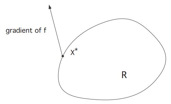
Case 2:
lies on We look at the direction of the vector . A geometric picture like Figure above is impossible; for if it were so, then would be greater that for some other point . So it must be is perpendicular to at (Suppose not perpendicular, then there exists a unit vector in the tangential direction s.t. , and this is the direction derivative) Since is perpendicular to (gradient is the fastest change direction, so normal to perpendicular), it follows that is parallel to . Therefore for some real number
, called a Lagrange multiplier. 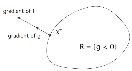
Critique
The foregoing argument is in fact incomplete, since we implicitly assumed that
If instead
The correct statement is this:
There exist real numbers
If
4.3 Statemet of Pontryagin Maximum Principle
We come now to the key assertion of this chapter, the theoretically interesting and practically useful theorem that if
We quote Francis Clarke [C2]: “The maximum principle was, in fact, the culmination of a long search in the calculus of variations for a comprehensive multiplier rule, which is the correct way to view it:
4.3.1 Fixed Time, Free Endpoint Problem
Let us review the basic set-up for our control problem.
We are given
Then given
We also introduce the payoff functional (To show the influence of free endpoint)
where the terminal time
Basic Problem
Find a control
The Pontryagin Maximum Principle, stated below, asserts the existence of a function
Definition
The control theory Hamiltonian is the function
Theorem 4.3 (Pontryagin Maximum Principle)
Assume
Then there exists a function
and
In addition,
Finally, we have the terminal condition
Remarks and Intepretations
The identities (ADJ) are the adjoint equations and (M) the maximization principle. Notice that (ODE) and (ADJ) resemble the structure of Hamilton's equations, discussed in §4.1. We also call (
) the transversality condition and will discuss its significance later. More precisely, formula (ODE) says that for
, we have
which is just the original equation of motion. Likewise, (ADJ) says
4.3.2 Free Time, Fixed Endpoint Problem
Let us next record the appropriate form of the Maximum Principle for a fixed endpoint problem.
As before, given a control
Assume now that a target point
Here
As before, the basic problem is to find an optimal control
Define the Hamiltonian
Theorem 4.4 (Pontryagin Maximum Principle)
Assume
Then there exists a function
and
Also,
Here
Remark and Warning
More precisely, we should define
A more careful statement of the Maximum Principle says "there exists a constant
- If
, we can renormalize to get , as we have done above. - If
, then does not depend on running payoff and in this case the Pontryagin Maximum Principle is not useful. This is a so-called "abnormal problem".
Compare these comments with the critique of the usual Lagrange multiplier method at the end of §4.2, and see also the proof in §A. 5 of the Appendix.
4.4 Application and Examples
How to Use the Maximum Principle
We mentioned earlier that the costate
Calculations with Lagrange multipliers
Recall our discussion in §4.2 about finding a point
Calculations with the costate
This same principle is valid for our much more complicated control theory problems: it is usually best not just to look for an optimal control
The following examples show how this works in practice, in certain cases for which we can actually solve everything explicitly or, failing that, at least deduce some useful information.
4.4.1 Example 1: Linear Time-Optimal Control.
For this example, let
for the payoff functional
where
In §3.2 we introduced the Hamiltonian
4.4.2 Example 2: Control of Production and Consumption
We return to Example 1 in Chapter 1, a model for optimal consumption in a simple economy. Recall that
We have the constraint
where
How can we characterize an optimal control
Introducing the maximum principle
We apply Pontryagin Maximum Principle, and to simplify notation we will not write the superscripts
and therefore
The dynamical equation is
and the adjoint equation is
The terminal condition reads
Lastly, the maximality principle asserts
Using the maximum principle
We now deduce useful information from (ODE), (ADJ), (M) and (T).
According to (M), at each time
Hence if we know
Since
But for times
Since
Restoring the superscript * to our notation, we consequently deduce that an optimal control is
for the optimal switching time
We leave it as an exercise to compute the switching time if the growth constant
4.4.3 Example 3: A Simple Linear-Quadratic Regulator
We take
with the quadratic cost functional
which we want to minimize. So we want to maximize the payoff functional
For this problem, the values of the controls are not constrained; that is,
Introducing the maximum principle
To simplify notation further we again drop the superscripts *. We have
and hence
The maximality condition becomes
We calculate the maximum on the right hand side by setting
The dynamical equations are therefore
and
Moreover
Using the Maximum Principle
So we must look at the system of equations
the general solution of which is
Since we know
Feedback controls
An elegant way to do so is to try to find optimal control in linear feedback form; that is, to look for a function
We henceforth suppose that an optimal feedback control of this form exists, and attempt to calculate
whence
so that
We will next discover a differential equation that
and recall that
Therefore
Since
This is called the Riccati equation.
In summary so far, to solve our linear-quadratic regulator problem, we need to first solve the Riccati equation
How to solve the Riccati equation. It turns out that we can convert (
for a function
Hence
and consequently
This is a terminal-value problem for second-order linear ODE, which we can solve by standard techniques. We then set
We will generalize this example later to systems, in §5.2.
4.4.4 Example 4: Moon Lander
This is a much more elaborate and interesting example, already introduced in Chapter 1.
Introduce the notation
The thrust is constrained so that
The dynamics are
with initial conditions
The goal is to land on the moon safely, maximizing the remaining fuel
This is so since
Introducing the maximum principle
In terms of the general notation, we have
Hence the Hamiltonian is
We next have to figure out the adjoint dynamics
Therefore
The maximization condition
Thus the optimal control law is given by the rule:
Using the maximum principle
Now we will attempt to figure out the form of the solution, and check it accords with the Maximum Principle.
Let us start by guessing that we first leave rocket engine of (i.e., set
Therefore, for times
with
Now put
Suppose the total amount of fuel to start with was
and so
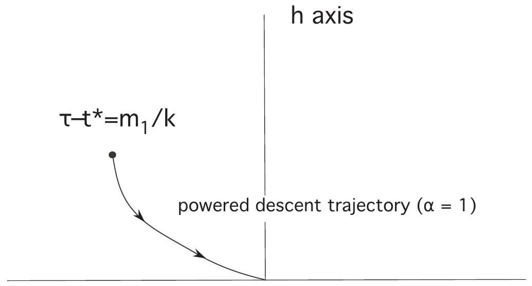
and thus
We combine the formulas for
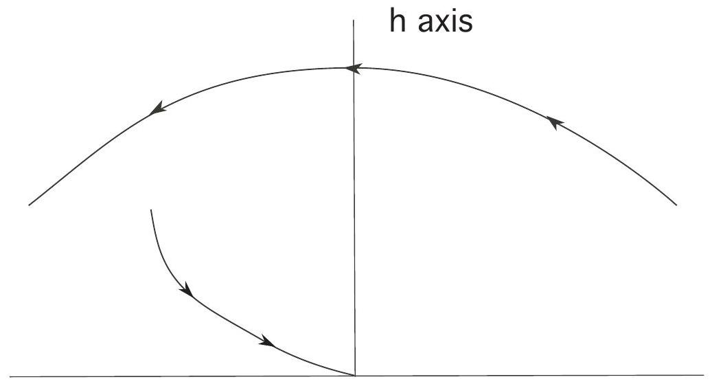
We deduce that the freefall trajectory
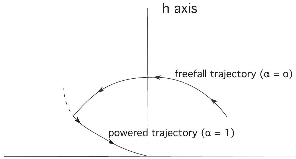
If we then move along this parabola until we hit the soft-landing curve from the previous picture, we can then turn on the rocket engine and land safely.
In the second case illustrated below, we miss switching curve, and hence cannot land safely on the moon switching once.
To justify our guess about the structure of the optimal control, let us now find the costate
We solve
Define
then
Choose
and then adjust
Thus an optimal control changes just once from 0 to 1 ; and so our earlier guess of
4.5 Maximum Principle with Transversality Conditions
Consider again the dynamics
In this section we discuss another variant problem, one for which the initial position is constrained to lie in a given set
So in this model we get to choose the starting point
where
Notation
We will assume that
Theorem 4.5 (More Transversality Conditions)
Let
Then there exists a function
We call
Remarks and Intepretations
- If we have
fixed and
then
in agreement with our earlier form of the terminal/transversality condition.
- Suppose that the surface
is the graph . Then says that belongs to the "orthogonal complement" of the subspace . But orthogonal complement of is the span of . Thus
for some unknown constants
4.6 More Applications
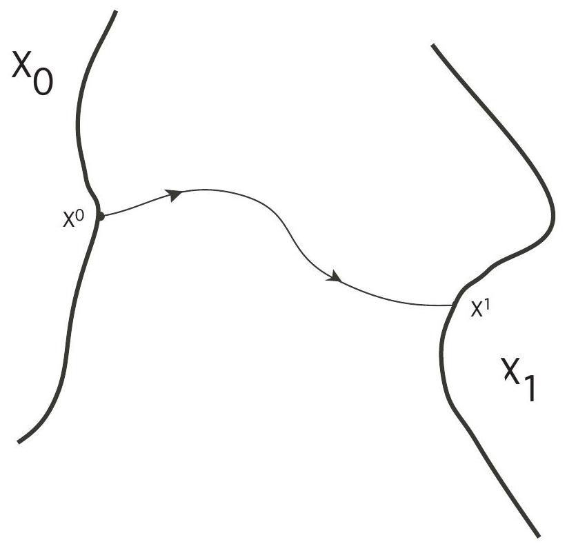
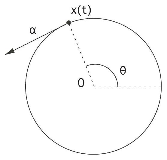
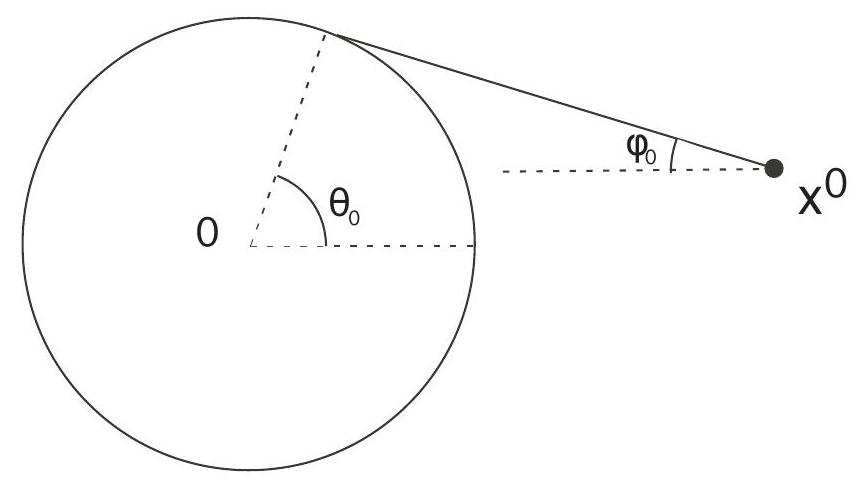
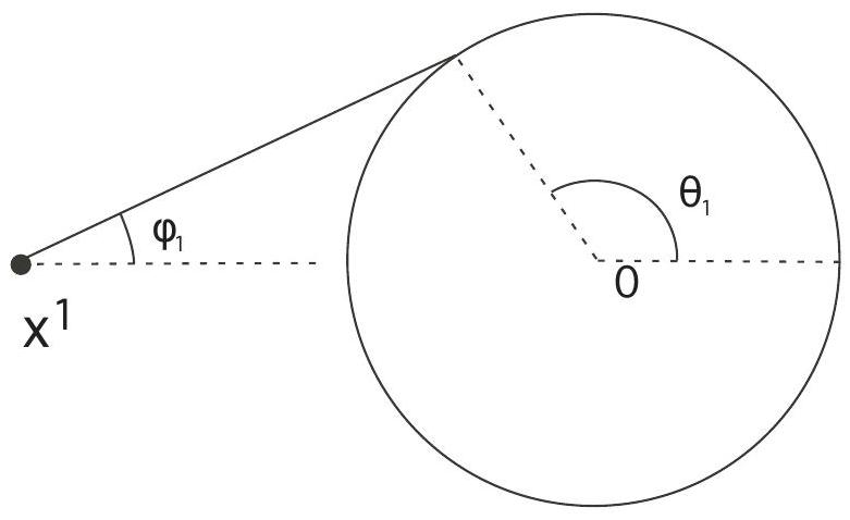
4.6.1 Example 1: Distance between Two Sets
As a first and simple example, let
for
We take
We want to minimize the length of the curve and, as a check on our general theory, will prove that the minimum is of course a straight line.
Using the maximum principle
We have
The adjoint dynamics equation
and therefore
The maximization principle ( M ) tells us that
The right hand side is maximized by
Finally, the transversality conditions say that
In other words,
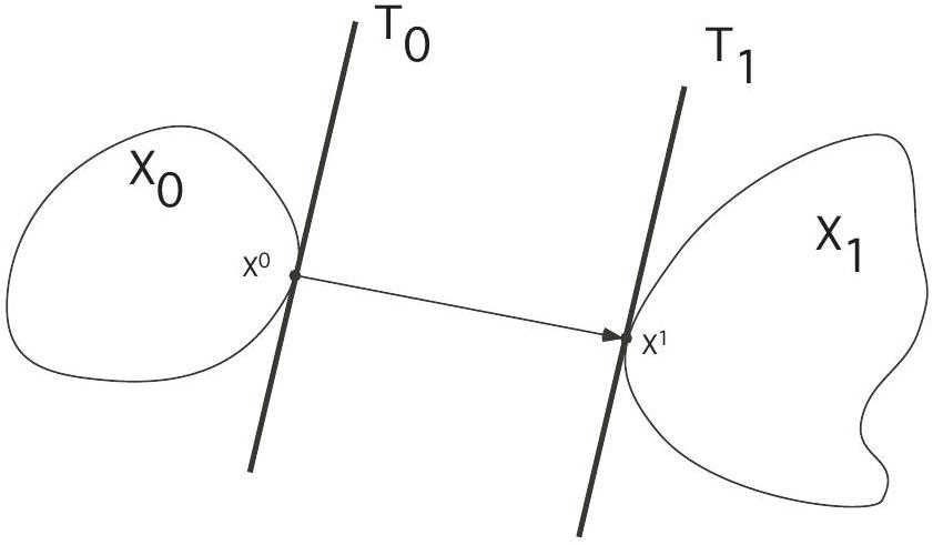
Now all of this is pretty obvious from the picture, but it is reassuring that the general theory predicts the proper answer.
4.6.2 Example 2: Commodity Trading
Next is a simple model for the trading of a commodity, say wheat. We let
We suppose that the price of wheat
where
Our intention is to maximize our holdings at the end time
The evolution is
This is a nonautonomous (
Using the maximum principle
What is our optimal buying and selling strategy? First, we compute the Hamiltonian
since
with the terminal condition
In our case
We then can solve for the costate:
The maximization principle
So
for
Critique
In some situations the amount of money on hand
4.7 Maximum Principle with State Constraints
We return once again to our usual setting:
for
State Constraints
We introduce a new complication by asking that our dynamics
for a given function
Definition
It will be convenient to introduce the quantity
Notice that if
Theorem 4.6 (Maximum Principle with State Constraints)
Let
Then there exists a costate function
and
To keep things simple, we have omitted some technical assumptions really needed for the Theorem to be valid.
Remarks and Intepretations
- Let
be of this form:
for given functions
The function
- Jump conditions. In the situation above, we always have
where
However,
this says there is (possibly) a jump in
4.8 More Applications
4.8.1 Example 1: Shortest Distance between Two Points, Avoiding An Obstacle.
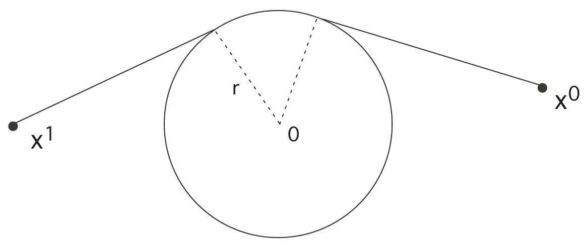
What is the shortest path between two points that avoids the disk
Let us take
for
We have
Case 1: avoiding the obstacle
Assume
Hence
Condition
The maximum occurs for
and therefore
Case 2: touching the obstacle
Suppose now
First we must calculate
Then
Now condition
which is to say,
Next, we employ the maximization principle
subject to the requirements that
that is,
We can combine these identities to eliminate
But we also know
and
hence
Solving for the unknowns. We now have the five equations
and
for some constant
Case 3: approaching and leaving the obstacle
In general, we must piece together the results from Case 1 and Case 2. So suppose now
We have shown that for times
for the angle
By the jump conditions,
These identities hold if and only if
The second equality says that the optimal trajectory is tangent to the disk
We turn next to the trajectory as it leaves
Now our formulas above for
for
Therefore
and so the trajectory is tangent to
Thus
and so
Critique
We have carried out elaborate calculations to derive some pretty obvious conclusions in this example. It is best to think of this as a confirmation in a simple case of Theorem 4.6, which applies in far more complicated situations.
4.8.2 An Inventory Control Model
Now we turn to a simple model for ordering and storing items in a warehouse. Let the time period
Our goal is to fill all customer orders shipped from our warehouse, while keeping our storage and ordering costs at a minimum. Hence the payoff to be maximized is
We have
Guessing the optimal strategy
Let us just guess the optimal control strategy: we should at first not order anything (
Using the maximum principle
We will prove this guess is right, using the Maximum Principle. Assume first that
and
Thus
If
According to
Thus
and
We have
But
and so
4.9 Numerical Solution of the Two Point Boundary Value Problem (TPBVP)
Reference: Chapter 12.6 in Numerical Optimal Control by Moritz Diehl and Sebastien Gros
At first, give the main drawbacks of the indirect approach:
- it must be possible to eliminate the controls from the problem by algebraic manipulations, which is not always straightforward or might even be impossible;
- the optimal controls might be a discontinuous function of
and , such that the BVP is possibly given by a non-smooth differential equation; - the differential equation might become very nonlinear and unstable and not suitable for a forward simulation.
All these issues of the indirect approach can partially be addressed, and most importantly, it offers an exact and elegant characterization of the solution of optimal control problems in continuous time.
In this section we address the question of how we can compute a solution of the boundary value problem (BVP) in the indirect approach. The remarkable observation is that the only non-trivial unknown is the initial value for the adjoints,
Using the shorthands
and
the system of equations can be summarized as:
This BVP has the
4.9.1 Single shooting
Single shooting starts with the following idea: for any guess of the initial value
For nonlinear dynamics
for some adequate step-size
In some cases, as said above, the forward simulation of the combined ODE might be an ill-conditioned problem so that single shooting cannot be employed. Even if the forward simulation problem is well-defined, the region of attraction of the Newton iteration on
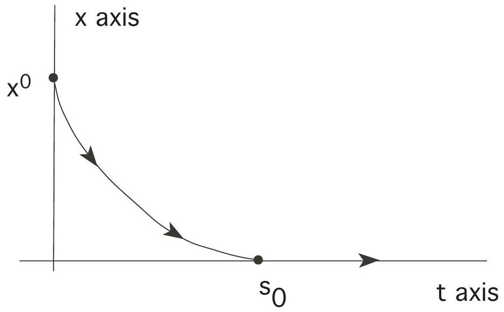
Example 4.9.1
We consider the optimal control problem:
with
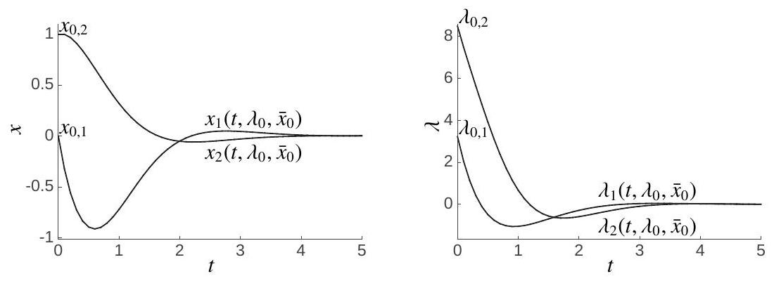
Figure 4.9.1: Illustration of the state and co-state trajectories for example 4.9.1 at the solution delivering
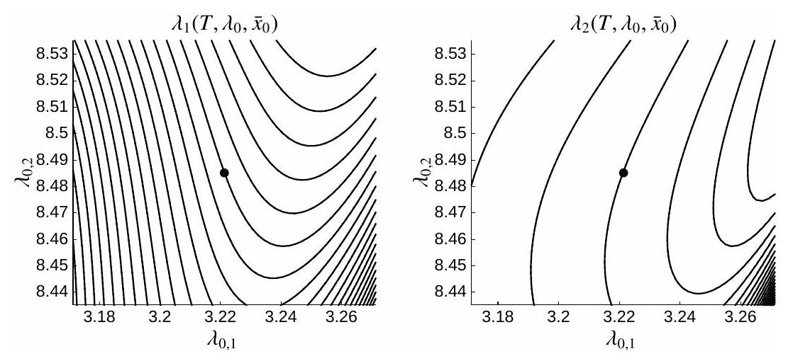
Figure 4.9.2: Illustration of the map
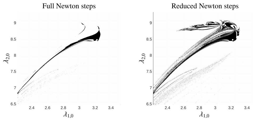
Figure 4.9.3: Illustration of the region of convergence of the Newton iteration
A crucial observation that will motivate an alternative to the single-shooting approach is illustrated in Figure 4.9.4, where the map
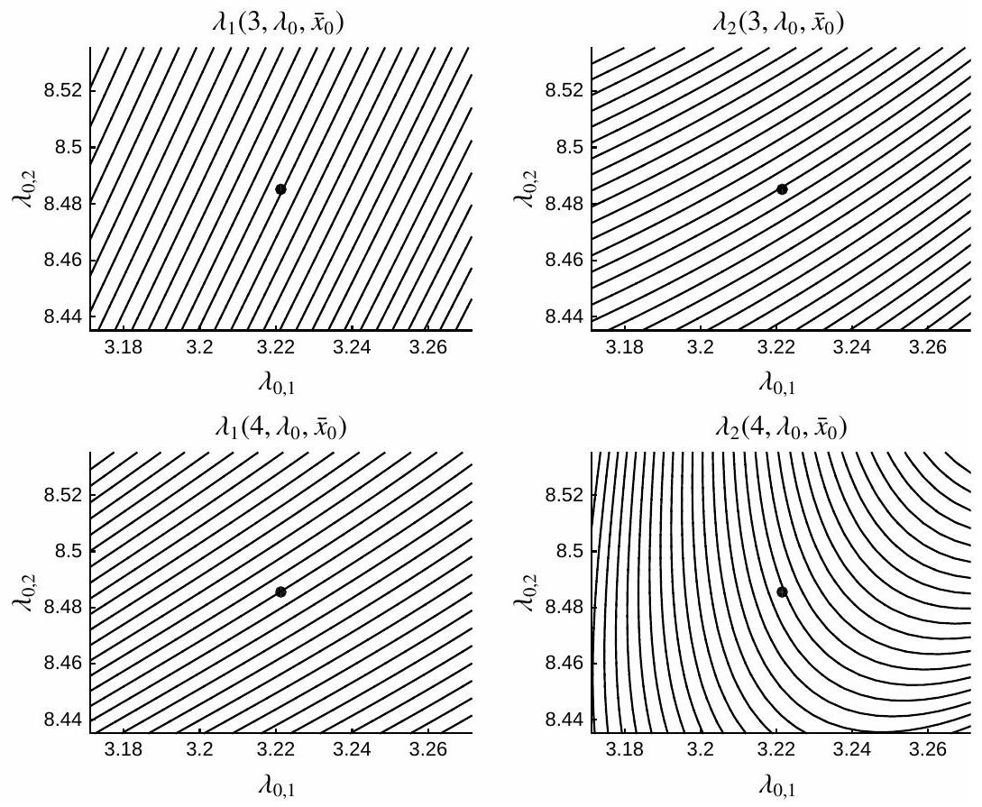
Figure 4.9.4: Illustration of the map
4.9.2 Multiple shooting
The nonlinearity of the integration map
for
One can then rewrite the conditions (4.6) altogether as the function:
where we note
for some step-size
Example 4.9.2
We consider the optimal control problem
We illustrate the Multiple-Shooting procedure (12.14) in Figure 4.9.5 for
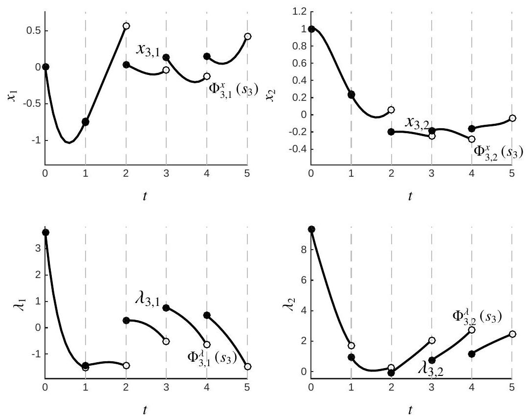
Figure 4.9.5: Illustration of the state and co-state trajectories for problem
One ought to observe that the time intervals
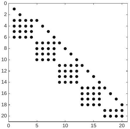
Figure 4.9.6: Illustration of sparsity pattern of the Jacobian matrix
It is important to observe that the set of algebraic conditions
The second alternative to single-shooting is the object of the next section, and can be construed as an extreme case of Multiple-Shooting. We detail this next.
4.9.3 Collocation & Pseudo-spectral methods
The second alternative approach to single shooting is to use simultaneous collocation or Pseudo-spectral methods. As we will see next, the two approaches are fairly similar. The key idea behind these methods is to introduce all the variables involved in processing the integration of the dynamics, and the related algebraic conditions into the set of algebraic equations to be processed.
The most common implementation of this idea is based on the Orthogonal Collocation method.
We consider the collocation-based integration of the state-costate dynamics on a time interval
where
The integration is then based on solving a set of collocation equations:
for
One can observe that equations
This elimination does not modify the behavior of the Newton iteration. We can gather the algebraic conditions
where
for some step-size
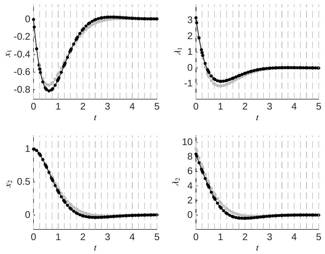
Figure 4.9.7: Illustration of the state and co-state trajectories for example 4.9.1 using the orthogonal collocation approach with
Example 4.9.3
We consider the optimal control problem from Example 4.9.1 with
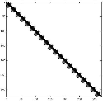
Figure 4.9.8: Illustration of the sparsity structure for the Jacobian
Pseudo-spectral methods
Pseudo-spectral methods deploy a very similar approach to the one described here, to the exception that they skip the division of the time interval
where