Functions and Linear Transformations and Matrices

Addendic B: Functions

function

If $A$ and $B$ are sets, then a function $f$ from $A$ to $B$, written $f:A\to B$, is a rule that associates to each element $x$ in $A$ a unique element denoted $f(x)$ in $B$. The element $f(x)$ is called the image of $x$ (under $f$), and $x$ is called a preimage of $f(x)$ (under $f$).

If $f:A\to B$, then $A$ is called the domain of $f$, $B$ is called the codomain of $f$, and the set $\{f(x):x\in A\}$ is called the range of f. Note that the range of $f$ is a subset of $B$. If $S\subseteq A$, we denote by $f(S)$ the set $\{f(x):x\in S\}$ of all images of elements of $S$. Likewise, if $T\subseteq B$, we denote by $f^{-1}(T)$ the set $\{x\in A:f(x)\in T\}$ of all preimages of elements in $T$.

Finally, two functions $f:A\to B$ and $g:A\to B$ are equal, written $f=g$, if $f(x)=g(x)$ for all $x\in A$.

Example B.1

Suppose that $A=[-10,10]$. Let $f:A\to R$ be the functio that assignss to each element $x$ in $A$ the element $x^2+1$ in $R$; that is, $f$ is defined by $f(x)=x^2+1$.

Then $A$ is the domain of $f$, $R$ is the codmain of $f$, and $[1,101]$ is the range of $f$. Since $f(2)=5$, the image of $2$ is $5$, and $2$ is a preimage of $5$. Notice that $-2$ is another preimage of $5$. Moreover, if $S=[1,2]$ and $T=[82,101]$, then $f(S)=[2,5]$ and $f^{-1}(T)=[-10,-9]\cup [9,10]$.

one-to-one, onto

As example 1 shows, the preimage of an element in the range need not be unique. Functions s.t. each element of the range has a unique preimage are called one-to-one (injective); that is $f:A\to B$ is one-to-one if $f(x)=f(y)$ implies $x=y$ or, equivalently, if $x\ne y$ implies $f(x)\ne f(y)$.

If $f:A\to B$ is a function with range $B$, that is, if $f(A)=B$, then $f$ is called onto (surjective).So $f$ is onto iff the range of $f$ equals the codomain of $f$. [core]

one-to-one + onto = bijective

Let $A,B,C$ be sets and $f:A\to B$ and $g:B\to C$ be functios. By following $f$ with $g$, we obtain a function $g\circ f:A\to C$ called the composite of $g$ and $f$. Thus $(g\circ f)(x)=g(f(x)),\mathrm{\forall }x\in A$.

• For example, let $A=B=C=R,f(x)=\sin x$, and $g(x)=x^2+3$. Then $(g\circ f)(x)=(g(f(x)))={\sin }^{2}x+3$, whereas $(f\circ g)(x)=f(g(x))=f(g(x))=\sin (x^2+3)$. Hence, $g\circ f\ne f\circ g$.
• Functionalcomposition is associative, i.e. if $h:C\to D$ is another function, then $h\circ (g\circ f)=(h\circ g)\circ f$.

A function $f:A\to B$ is said to e invertible if there exists a function $g:B\to A$ s.t. $(f\circ g)(y)=y,\mathrm{\forall }y\in B$ and $(g\circ f)(x)=x,\mathrm{\forall }x\in A$. If such a function $g$ exists, then it's unique and is called the inverse of $f$. We denote the inverse of $f$ (when it exists) by $f^{-1}$. It can be shown that $f$ is invertible iff $f$ is both one-to-one and onto.

The following facts about invertible functions are easily proved:

1. If $f:A\to B$ is invertible, then $f^{-1}$ is invertible, and $(f^{-1}{)}^{-1}=f$.
2. If $f:A\to B$ and $g:B\to C$ ar invertible, then $g\circ f$ is invertible, and $(g\circ f{)}^{-1}=f^{-1}\circ g^{-1}$.

2.1 Linear Transformations, Null Spaces, and Ranges

Linear Transformation

Now it's natural to consider those functions defined on vector spaces that in some sense "preserve" the structure.

Definition: linear transformation

Let $\mathsf{V}\mathsf{,}\mathsf{W}$ be vector spaces (over $F$). We call a function $\mathsf{T}:\mathsf{V}\to \mathsf{W}$ a linear transformation from $\mathsf{V}$ to $\mathsf{W}$ if, $\mathrm{\forall }x,y\in \mathsf{V}$ and $c\in F$, we have

• $\mathsf{T}(x+y)=\mathsf{T}(x)+\mathsf{T}(y)$ (additivity)
• $\mathsf{T}(cx)=c\mathsf{T}(x)$ (scaling)

Often simply all $\mathsf{T}$ linear. Following are properties of a function: $\mathsf{T}:\mathsf{V}\to \mathsf{W}$:

Properties

1. If $\mathsf{T}$ is linear, then $\mathsf{T}(0)=0$;
2. $\mathsf{T}$ is linear iff $\mathsf{T}(cx+y)=c\mathsf{T}(x)+\mathsf{T}(y),\mathrm{\forall }x,y\in \mathsf{V}$ and $c\in F$; (Generally used to prove that a given transformation is linear)[core]
3. If $\mathsf{T}$ is linear, then $\mathsf{T}(x-y)=\mathsf{T}(x)-\mathsf{T}(y),\mathrm{\forall }x,y\in \mathsf{V}$;
4. $\mathsf{T}$ is linear iff for $x_1,x_2,\cdots ,x_n\in \mathsf{V}$ and $a_1,a_2,\cdots ,a_n\in F$, we have

$$\mathsf{T}\left(\sum _{i=1}^n{a}_i{x}_i\right)=\sum _{i=1}^n{a}_i\mathsf{T}(x_i).$$

Example 1

Define

$$\mathsf{T}:{\mathbb{R}}^2\to {\mathbb{R}}^2\text{ by }\mathsf{T}(a_1,a_2)=(2a_1+a_2,a_1).$$

To show that $\mathsf{T}$ is linear, let $c\in R$ and $x,y\in {\mathbb{R}}^2$, where $x=(b_1,b_2)$ and $y=(d_1,d_2)$. Since

$$cx+y=(c{b}_1+d_1,c{b}_2+d_2)$$

we have

$$\mathsf{T}(cx+y)=(2(c{b}_1+d_1)+c{b}_2+d_2,c{b}_1+d_1).$$

Also

$$\begin{array}{rl}c\mathrm{\top }(x)+\mathrm{\top }(y)& =c(2b_1+b_2,b_1)+(2d_1+d_2,d_1)\\ & =(2c{b}_1+c{b}_2+2d_1+d_2,c{b}_1+d_1)\\ & =(2(c{b}_1+d_1)+c{b}_2+d_2,c{b}_1+d_1).\end{array}$$

So $\mathsf{T}$ is linear.

Example 2: rotation

For any angle $\theta$, define ${\mathsf{T}}_{\theta }:{\mathbb{R}}^2\to {\mathbb{R}}^2$ by the rule: ${\mathsf{T}}_{\theta }(a_1,a_2)$ is the vector obtained by rotating $(a_1,a_2)$ counterclockwise by $\theta$ if $(a_1,a_2)\ne (0,0)$, and ${\mathsf{T}}_{\theta }(0,0)=(0,0)$.

Then ${\mathsf{T}}_{\theta }:{\mathbb{R}}^2\to {\mathbb{R}}^2$ is a linear transformation that is called the rotation by $\theta$.

We determine an explicit formula for ${\mathsf{T}}_{\theta }$. Fix a nonzero vector $(a_1,a_2)\in {\mathbb{R}}^2$. Let $\alpha$ be the angle that $(a_1,a_2)$ makes with the positive $x$-axis, and let $r=\sqrt{a_1^2+a_2^2}$. Then $a_1=r\cos \alpha$ and $a_2=r\sin \alpha$. Also, ${\mathsf{T}}_{\theta }(a_1,a_2)$ has length $r$ and makes an angle $\alpha +\theta$ with the positive $x$-axis. It follows that

$$\begin{array}{rl}{\mathsf{T}}_{\theta }(a_1,a_2)& =(r\cos (\alpha +\theta ),r\sin (\alpha +\theta ))\\ & =(r\cos \alpha \cos \theta -r\sin \alpha \sin \theta ,r\cos \alpha \sin \theta +r\sin \alpha \cos \theta )\\ & =(a_1\cos \theta -a_2\sin \theta ,a_1\sin \theta +a_2\cos \theta )\end{array}$$

Finally, observe that this same formula is valid for $(a_1,a_2)=(0,0)$. It is now easy to show, as in Example 1, that ${\mathsf{T}}_{\theta }$ is linear.

Example 3&4: Reflection

Define $\mathsf{T}:{\mathbb{R}}^2\to {\mathbb{R}}^2$ by $\mathsf{T}(a_1,a_2)=(a_1,-a_2)$. $\mathsf{T}$ is called the reflection about the x-axis

Define $\mathsf{T}:{\mathbb{R}}^2\to {\mathbb{R}}^2$ by $\mathsf{T}(a_1,a_2)=(-a_1,a_2)$. $\mathsf{T}$ is called the reflection about the y-axis

Example 5: Polynominal

Define $\mathsf{T}:{\mathsf{P}}_n(\mathbb{R})\to {\mathsf{P}}_{n-1}(\mathbb{R})$ by $\mathsf{T}(f(x))=f^{\prime }(x)$, where $f^{\prime }(x)$ denotes the derivative of $f(x)$. To show that $\mathsf{T}$ is linear, let $g(x),h(x)\in {\mathsf{P}}_n(\mathbb{R})$ and $a\in \mathbb{R}$. Now

$$\mathsf{T}(ag(x)+h(x))=(ag(x)+h(x){)}^{\prime }=a{g}^{\prime }(x)+h^{\prime }(x)=a\mathsf{T}(g(x))=\mathsf{T}(h(x)).$$

So by property 2 above, $\mathsf{T}$ is linear.

Example 6: integration

Let $\mathsf{V}=\mathsf{C}(\mathbb{R})$, the vector space of continous real-valued functions on $\mathbb{R}$. Let $a,b\in \mathbb{R},a<b$. Define $\mathsf{T}:\mathsf{V}\to \mathbb{R}$ by

$$\mathsf{T}(f)={\int }_a^{b}f(t)\mathrm{d}t.$$

for all $f\in \mathsf{V}$. Then $\mathsf{T}$ is a linear transformation because the definte integral of a linear combination of functions is the same as the linear combination f he definite integrals of the fnctions.

Special transformations

For vector spaces $\mathsf{V}\mathsf{,}\mathsf{W}$ (over $F$), we define the identity transformation ${\mathsf{I}}_{\mathsf{V}}:\mathsf{V}\to \mathsf{V}$ by ${\mathsf{I}}_{\mathsf{V}}(x)=x,\mathrm{\forall }x\in \mathsf{V}$ and the zero transformation$T_0:\mathsf{V}\to \mathsf{W}$ by ${\mathsf{T}}_0(x)=0$ for all $x\in \mathsf{V}$. It is clear that both of these transformations are linear. We often write $\mathsf{I}$ instead of ${\mathsf{I}}_{\mathsf{V}}$.

We now turn our attention to two very important sets associated with linear transformations: the range and null space. The determination of these sets allows us to examine more closely the intrinsic properties of a linear transformation.

Definitions: null space/kerne; range / image [core]

Let $\mathsf{V}\mathsf{,}\mathsf{W}$ be vector spaces, and let $\mathsf{T}:\mathsf{V}\to \mathsf{W}$ be linear. We define the null space (or kernel) $\mathsf{N}\mathsf{(}\mathsf{T}\mathsf{)}$ of $\mathsf{T}$ to be the set of all vectors $x$ in $\mathsf{V}$ s.t. $\mathsf{T}(x)=0$; i.e., $\mathsf{N}\mathsf{(}\mathsf{T}\mathsf{)}=\{x\in \mathsf{V}:\mathsf{T}(x)=0\}$.

We define the range (or image) $\mathsf{R}\mathsf{(}\mathsf{T}\mathsf{)}$ of $\mathsf{T}$ to be the subset of $\mathsf{W}$ consisting of all images (under $\mathsf{T}$) of vectors in $\mathsf{V}$; i.e., $\mathsf{R}\mathsf{(}\mathsf{T}\mathsf{)}=\{\mathsf{T}(x):x\in \mathsf{V}\}$.

Example 7: identity and zero transformation

Let $\mathsf{V}\mathsf{,}\mathsf{W}$ be vector spaces, and let $\mathsf{I}:\mathsf{V}\to \mathsf{V}$ and ${\mathsf{T}}_0:\mathsf{V}\to \mathsf{W}$ be the identity and zero transformation, respectively. Then $\mathsf{N}\mathsf{(}\mathsf{I}\mathsf{)}=\{0\},\mathsf{R}\mathsf{(}\mathsf{I}\mathsf{)}\mathsf{=}\mathsf{V},\mathsf{N}({\mathsf{T}}_0)=\mathsf{V},\mathsf{R}({\mathsf{T}}_0)=\{0\}$

Example 8

Let $\mathsf{T}:{\mathbb{R}}^3\to {\mathbb{R}}^2$ be the linear transformation defined by

$$\mathsf{T}(a_1,a_2,a_3)=(a_1-a_2,2a_3).$$

It's easy to verify that:

$$\mathsf{N}\mathsf{(}\mathsf{T}\mathsf{)}=\{(a,a,0):a\in \mathbb{R}\},\text{ and }\mathsf{R}\mathsf{(}\mathsf{T}\mathsf{)}={\mathbb{R}}^2.$$

Theorem 2.1

Let $\mathsf{V}\mathsf{,}\mathsf{W}$ be vector spaces and $\mathsf{T}:\mathsf{V}\to \mathsf{W}$ be linear. Then $\mathsf{N}\mathsf{(}\mathsf{T}\mathsf{)}$ and $\mathsf{R}\mathsf{(}\mathsf{T}\mathsf{)}$ are subspaces of $\mathsf{V}\mathsf{,}\mathsf{W}$, respectively.

Theorem 2.2

Let $\mathsf{V}\mathsf{,}\mathsf{W}$ be vector spaces and $\mathsf{T}:\mathsf{V}\to \mathsf{W}$ be linear. If $\beta =\{v_1,v_2\cdots ,v_n\}$ is a basis for $\mathsf{V}$, then

$$\mathsf{R}\mathsf{(}\mathsf{T}\mathsf{)}=\mathrm{span}(\mathsf{T}(\beta ))=\mathrm{span}(\{\mathsf{T}(v_1),\mathsf{T}(v_2),\cdots ,\mathsf{T}(v_n)\}).$$

Recall Theorem 1.5 in §1 that the relation between subspace and span.

Example 9

Define the linear transformation $\mathsf{T}:{\mathsf{P}}_2(\mathbb{R})\to {\mathsf{M}}_{2\times 2}(\mathbb{R})$ by

$$\mathsf{T}(f(x))=\left(\begin{array}{cc}f(1)-f(2)& 0\\ 0& f(0)\end{array}\right)$$

Since $\beta =\{1,x,x^2\}$ is a basis for ${\mathsf{P}}_2(\mathbb{R})$, we have

$$\begin{array}{rl}\mathsf{R}(\mathsf{T})& =\mathrm{span}(\mathsf{T}(\beta ))=\mathrm{span}(\{\mathsf{T}(1),\mathsf{T}(x),\mathsf{T}(x^2)\})\\ & =\mathrm{span}\left(\{\left(\begin{array}{cc}0& 0\\ 0& 1\end{array}\right),\left(\begin{array}{cc}-1& 0\\ 0& 0\end{array}\right),\left(\begin{array}{cc}-3& 0\\ 0& 0\end{array}\right)\}\right)\\ & =\mathrm{span}\left(\{\left(\begin{array}{cc}0& 0\\ 0& 1\end{array}\right),\left(\begin{array}{cc}-1& 0\\ 0& 0\end{array}\right)\}\right)\end{array}$$

Thus, we have found a basis for $\mathsf{R}\mathsf{(}\mathsf{T}\mathsf{)}$, so $\dim (\mathsf{R}\mathsf{(}\mathsf{T}\mathsf{)})=2$.

Definition and Theorem

As in §1.4, we measure the "size" of a subspace by its dimension. The null space and range are so important that we attach special names to their respective dimensions.

Definition: nulity; rank [core]

Let $\mathsf{V}$ and $\mathsf{W}$ be vector spaces, and let $T:\mathsf{V}\to \mathsf{W}$ be linear. If $\mathsf{N}\mathsf{(}\mathsf{T}\mathsf{)}$ and $\mathsf{R}\mathsf{(}\mathsf{T}\mathsf{)}$ are finite-dimensional, then we define:

• Nullity of $\mathsf{T}$, denoted $\mathrm{nullity}(\mathsf{T})$, as the dimension of $\mathsf{N}\mathsf{(}\mathsf{T}\mathsf{)}$.
• Rank of $\mathsf{T}$, denoted $\mathrm{rank}(\mathsf{T})$, as the dimension of $\mathsf{R}\mathsf{(}\mathsf{T}\mathsf{)}$.

Theorem 2.3: Dimension Theorem [core]

Let $\mathsf{V}$ and $\mathsf{W}$ be vector spaces, and $\mathsf{T}:\mathsf{V}\to \mathsf{W}$ linear. If $\mathsf{V}$ is finite-dimensional, then

$$\mathrm{nullity}(\mathsf{T})+\mathrm{rank}(\mathsf{T})=\dim (\mathsf{V})$$

Theorem 2.4: Null Space and One-to-one [core]

Let $\mathsf{V}$ and $\mathsf{W}$ be vector spaces, and $\mathsf{T}:\mathsf{V}\to \mathsf{W}$ linear. Then $\mathsf{T}$ is one-to-one iff

$$\mathsf{N}\mathsf{(}\mathsf{T}\mathsf{)}=\{0\}$$

Theorem 2.5 [core]

Let $\mathsf{V}$ and $\mathsf{W}$ be finite-dimensional vector spaces of equal and finite dimension, and $\mathsf{T}:\mathsf{V}\to \mathsf{W}$ linear. The following are equivalent:

• $\mathsf{T}$ is one-to-one.
• $\mathsf{T}$ is onto.
• $\mathrm{rank}(\mathsf{T})=\dim (\mathsf{V})$.

Example 10

Let $\mathsf{T}:{\mathsf{P}}_2(\mathbb{R})\to {\mathsf{P}}_3(\mathbb{R})$ be the linear transformation defined by

$$\mathsf{T}(f(x))=2f^{\prime }(x)+{\int }_0^{x}3f(t)\mathrm{d}t$$

Now

$$\begin{array}{rl}\mathsf{R}\mathsf{(}\mathsf{T}\mathsf{)}& =\mathrm{span}(\{\mathsf{T}(1),\mathsf{T}(x),\mathsf{T}(x^2)\})\\ & =\mathrm{span}\left(\{3x,2+\frac{3}{2}{x}^2,4x+x^3\}\right).\end{array}$$

• Since $\mathrm{span}\left(\{3x,2+\frac{3}{2}{x}^2,4x+x^3\}\right)$ is linear independent, The rank is $3$;
• Since $\dim ({\mathsf{P}}_3(\mathbb{R}))=4,\mathsf{T}$ is not onto;
• From the dimension theorem, $\mathrm{nullity}(\mathsf{T})+3=3$, so nullity is $0$, and therefore $\mathsf{N}\mathsf{(}\mathsf{T}\mathsf{)}=\{0\}$.

So $\mathsf{T}$ is one-to-one but not onto.

Example 11

Let $\mathsf{T}:{\mathsf{F}}^2\to {\mathsf{F}}^2$ be the linear transformation defined by

$$\mathsf{T}(a_1,a_2)=(a_1+a_2,a_1)$$

It's easy to see that $\mathsf{N}\mathsf{(}\mathsf{T}\mathsf{)}=\{0\}$; so $\mathsf{T}$ is one-to-one. And Theorem 2.5 tells us that $\mathsf{T}$ must be onto.

Example 12

Let $T:{\mathsf{P}}_2(\mathbb{R})\to {\mathbb{R}}^3$ be the linear transformation defined by

$$\mathsf{T}(a_0+a_{1}x+a_2{x}^2)=(a_0,a_1,a_2)$$

Clearly $\mathsf{T}$ is linear and one-to-one. Let $S=\{1-x+3x^2,x+x^2,1-2x^2\}$. Then $S$ is linearly independent in ${\mathsf{P}}_2(\mathbb{R})$ because

$$\mathsf{T}(S)=\{(2,-1,3),(0,1,1),(1,0,-2)\}$$

is linearly independent in ${\mathbb{R}}^3$.

Theorem 2.6

Theorem 2.6

Let $\mathsf{V}$ and $\mathsf{W}$ be vector spaces over $F$, and suppose that $\{v_1,v_2,\cdots ,v_n\}$ is a basis for $\mathsf{V}$. For $w_1,w_2,\cdots ,w_n$ in $\mathsf{W}$, there exists exactly one linear transformation: $\mathsf{T}:\mathsf{V}\to \mathsf{W}$ s.t. $\mathsf{T}(v_i)=w_i$,for $i=1,2,\cdots ,n$.

Corollary

Let $\mathsf{V}$ and $\mathsf{W}$ be vector spaces, and suppose that $\mathsf{V}$ has a finite basis $\{v_1,v_2,\cdots ,v_n\}$. If $\mathsf{U}\mathsf{,}\mathsf{T}:\mathsf{V}\to \mathsf{W}$ are linear and $\mathsf{U}(v_i)=\mathsf{T}(v_i)$ for $i=1,2,\cdots ,n$, then $\mathsf{U}\mathsf{=}\mathsf{T}$.

Example 13

Let $\mathsf{T}:{\mathbb{R}}^2\to {\mathbb{R}}^2$ be the linear transformation defined by

$$\mathsf{T}(a_1,a_2)=(2a_2-a_1,3a_1).$$

and suppose that $\mathsf{U}:{\mathbb{R}}^2\to {\mathbb{R}}^2$ is linear. If we know that $\mathsf{U}(1,2)=(3,3)$ and $\mathsf{U}(1,1)=(1,3)$, then $\mathsf{U}\mathsf{=}\mathsf{T}$. This follows from the corollary and from the fact that $\{(1,2),(1,1)\}$ is the basis for ${\mathbb{R}}^2$.

2.2 The Matrix Representation of a Linear Transformations

coordinate vector

Definition: ordered basis

Let $\mathsf{V}$ be a finite-dimensional vector space. An ordered basis for $\mathsf{V}$ is a basis for $\mathsf{V}$ endowed with a specific order; that is, an ordered basis for $\mathsf{V}$ is a finite sequence of linearly independent vectors in $\mathsf{V}$ that generates $\mathsf{V}$.

Example 1

In ${\mathsf{F}}^3,\beta =\{e_1,e_2,e_3\}$ can be considered as ordered basis. Also $\gamma =\{e_2,e_1,e_3\}$ is an ordered basis, but $\beta \ne \gamma$ as ordered bases

For the vector space ${\mathsf{F}}^n$, we call $\{e_1,e_2,\cdots ,e_n\}$ the standard ordered basis for ${\mathsf{F}}^n$. Similarly, for the vector space ${\mathsf{P}}_n(F)$, we call $\{1,x,\cdots ,x^n\}$ the standard ordered basis for ${\mathsf{P}}_n(F)$.

Definition: coordinate vector

Let $\beta =\{v_1,v_2,···,v_n\}$ be an ordered basis for a finite-dimensional vector space $\mathsf{V}$. For $x\in \mathsf{V}$, let $a_1,a_2,\cdots ,a_n$ be the unique scalars s.t.

$$x=\sum _{i=1}^n{a}_i{u}_i$$

We define the coordinate vecotr of $x$ relative to $\beta$, denoted $[x{]}_{\beta }$ [core]. by

$$[x{]}_{\beta }=(a_1,a_2,\cdots ,a_n{)}^{\mathrm{\top }}.$$

Example 2: coordinate vector for polynominal

Let $\mathsf{V}={\mathsf{P}}_2(\mathbb{R})$, an let $\beta =\{1,x,x^2\}$ be the standard ordered basis for $\mathsf{V}$. If $f(x)=4+6x-7x^2$, then

$$[f{]}_{\beta }=(4,6,-7{)}^{\mathrm{\top }}.$$

matrix representation

Definition: matrix representation [core]

Using the notation above, we call the $m\times n$ matrix $A$ defined by $A_{ij}=a_{ij}$ the matrix representation of $\mathsf{T}$ in the ordered bases $\beta$ and $\gamma$ and write $A=[\mathsf{T}{]}_{\beta }^{\gamma }$ .

If $\mathsf{V}\mathsf{=}\mathsf{W}$ and $\beta =\gamma$, then we write $A=[\mathsf{T}{]}_{\beta }$.

Notice that the jth column of $A$ is simply $[\mathsf{T}(v_j){]}_{\gamma }$. Also observe that if $\mathsf{U}:\mathsf{V}\to \mathsf{W}$ is a linear transformation s.t. $[\mathsf{U}{]}_{\beta }^{\gamma }=[\mathsf{T}{]}_{\beta }^{\gamma }$, then $\mathsf{U}\mathsf{=}\mathsf{T}$ by the corollary to theorem 2.6.

Example 3: matrix representation for tuples

Let $\mathsf{T}:{\mathbb{R}}^2\to {\mathbb{R}}^3$ be defined by

$$\mathsf{T}(a_1,a_2)=(a_1+3a_2,0,2a_1-4a_2)$$

Let $\beta ,\gamma$ be the standard ordered bases for ${\mathbb{R}}^2$ and ${\mathbb{R}}^3$, respectively. Now

$$\mathsf{T}(1,0)=(1,0,2)=1e_1+0e_2+2e_3.$$

and

$$\mathsf{T}(0,1)=(3,0,-4)=3e_1+0e_2+-4e_3.$$

Hence

$$[\mathsf{T}{]}_{\beta }^{\gamma }=\left(\begin{array}{cc}1& 3\\ 0& 0\\ 2& -4\end{array}\right)$$

If we let ${\gamma }^{\prime }=\{e_3,e_2,e_1\}$, then

$$[\mathsf{T}{]}_{\beta }^{{\gamma }^{\prime }}=\left(\begin{array}{cc}2& -4\\ 0& 0\\ 1& 3\end{array}\right)$$

Example 4: matrix representation for polynominal

Let ${\mathsf{T}:\mathsf{P}}_3(\mathbb{R})\to {\mathsf{P}}_2(\mathbb{R})$ be the linear transformation defined by $\mathsf{T}(f(x))=f^{\prime }(x)$.Let $\beta ,\gamma$ be the standard ordered bases for ${\mathsf{P}}_3(\mathbb{R})$ and ${\mathsf{P}}_2(\mathbb{R})$, respectively. Then

$$\begin{array}{rl}\mathsf{T}(1)& =0\cdot 1+0\cdot x+0\cdot x^2\\ \mathsf{T}(x)& =1\cdot 1+0\cdot x+0\cdot x^2\\ \mathsf{T}(x^2)& =0\cdot 1+2\cdot x+0\cdot x^2\\ \mathsf{T}(x^3)& =0\cdot 1+0\cdot x+3\cdot x^2\end{array}$$

So

$$\left[\frac{\mathrm{d}}{\mathrm{d}x}\right]=[\mathsf{T}{]}_{\beta }^{\gamma }=\left(\begin{array}{cccc}0& 1& 0& 0\\ 0& 0& 2& 0\\ 0& 0& 0& 3\end{array}\right)$$

i.e.

$$\begin{array}{c}f(x)=a+bx+c{x}^2+d{x}^3\\ \mathsf{T}(f(x))=f^{\prime }(x)=b+2cx+3d{x}^2\\ \left[\begin{array}{c}b\\ 2c\\ 3d\end{array}\right]=\left[\begin{array}{cccc}0& 1& 0& 0\\ 0& 0& 2& 0\\ 0& 0& 0& 3\end{array}\right]\left[\begin{array}{c}a\\ b\\ c\\ d\end{array}\right]\end{array}$$

Note that when $\mathsf{T}(x^j)$ is written as a linear combination of the vectors of $\gamma$, its coefficients gives the entries of the jth column of $[\mathsf{T}{]}_{\beta }^{\gamma }$.

operations on linear transformation

Definition

Let $\mathsf{T}\mathsf{,}\mathsf{U}:\mathsf{V}\to \mathsf{W}$ be arbitary functions, where $\mathsf{V}\mathsf{,}\mathsf{W}$ are vector spaces over $F$, and let $a\in F$. We define:

• $\mathsf{T}\mathsf{+}\mathsf{U}:\mathsf{V}\to \mathsf{W}$ by $\mathsf{(}\mathsf{T}\mathsf{+}\mathsf{U}\mathsf{)}(x)=\mathsf{T}(x)+\mathsf{U}(x)$ for all $x\in \mathsf{V}$;
• $a\mathsf{T}:\mathsf{V}\to \mathsf{W}$ by $(a\mathsf{T})(x)=a\mathsf{T}(x)$ for all $x\in \mathsf{V}$;

Theorem 2.7

Let $\mathsf{V}\mathsf{,}\mathsf{W}$ be vector spaces over a field $F$, and let $\mathsf{T}\mathsf{,}\mathsf{U}:\mathsf{V}\to \mathsf{W}$ be linear.

• For all $a\in F,a\mathsf{T}\mathsf{+}\mathsf{U}$ is linear.
• Using the operations of addition andscalar multiplication in the precedingg definition, the collection of all linear transformation from $\mathsf{V}$ to $\mathsf{W}$ is a vector space over $F$.

Definition

Let $\mathsf{V}\mathsf{,}\mathsf{W}$ be vector spaces over $F$. We denote the vector space of all linear transformation from $\mathsf{V}$ to $\mathsf{W}$ by $\mathcal{L}(\mathsf{V}\mathsf{,}\mathsf{W})$. In the case that $\mathsf{V}\mathsf{=}\mathsf{W}$, we write $\mathcal{L}(\mathsf{V})$ instead of $\mathcal{L}(\mathsf{V}\mathsf{,}\mathsf{W})$.

Theorem 2.8

Let $\mathsf{V}\mathsf{,}\mathsf{W}$ be finite-dimensional vector spaces with ordered bases $\beta ,\gamma$, respectively, and let $\mathsf{T}\mathsf{,}\mathsf{U}:\mathsf{V}\to \mathsf{W}$ be linear transformations. Then

• $[\mathsf{T}\mathsf{+}\mathsf{U}{]}_{\beta }^{\gamma }=[\mathsf{T}{]}_{\beta }^{\gamma }+[\mathsf{U}{]}_{\beta }^{\gamma }$
• $[a\mathsf{T}{]}_{\beta }^{\gamma }=a[\mathsf{T}{]}_{\beta }^{\gamma }$ for all scalars $a$.

Example 5

Let $\mathsf{T}:{\mathbb{R}}^2\to {\mathbb{R}}^3$ and $\mathsf{U}:{\mathbb{R}}^2\to {\mathbb{R}}^3$ be the linear transformations respectively defined by

$$\begin{array}{rl}\mathsf{T}(a_1,a_2)& =(a_1+3a_2,0,2a_1-4a_2)\\ \mathsf{U}(a_1,a_2)& =(a_1-a_2,2a_1,3a_1+2a_2)\end{array}$$

Let $\beta ,\gamma$ be the standard ordered bases of ${\mathbb{R}}^2{\mathbb{R}}^3$, respectively. Then

$$[\mathsf{T}{]}_{\beta }^{\gamma }=\left(\begin{array}{cc}1& 3\\ 0& 0\\ 2& -4\end{array}\right)$$

(as completed in Example 3), and

$$[\mathsf{U}{]}_{\beta }^{\gamma }=\left(\begin{array}{cc}1& -1\\ 2& 0\\ 3& 2\end{array}\right)$$

If we compute $\mathsf{T}\mathsf{+}\mathsf{U}$ usingthe proceding definitions, we obtain

$$(\mathsf{T}\mathsf{+}\mathsf{U})(a_1,a_2)=(2a_1+2a_2,2a_1,5a_1-2a_2).$$

So

$$[\mathsf{T}\mathsf{+}\mathsf{U}{]}_{\beta }^{\gamma }=\left(\begin{array}{cc}2& 2\\ 2& 0\\ 5& -2\end{array}\right)$$

which is simply $[\mathsf{T}{]}_{\beta }^{\gamma }+[\mathsf{U}{]}_{\beta }^{\gamma }$, illustrated Theorem 2.8

2.3 Composition of Linear Transformations and Matrix Multiplication

matrix product

Theorem 2.9

Let $\mathsf{V}\mathsf{,}\mathsf{W}\mathsf{,}\mathsf{Z}$ be vector spaces over the same field $F$, and let $\mathsf{T}:\mathsf{V}\to \mathsf{W}$ and $\mathsf{U}:\mathsf{W}\to \mathsf{Z}$ be linear, then $\mathsf{U}\mathsf{T}:\mathsf{V}\to \mathsf{Z}$ is linear.

Theorem 2.10

Let $\mathsf{V}$ be a vector space. Let ${\mathsf{T}\mathsf{,}\mathsf{U}}_1,{\mathsf{U}}_2\in \mathcal{L}(\mathsf{V})$. Then

• $\mathsf{T}({\mathsf{U}}_1+{\mathsf{U}}_2)={\mathsf{TU}}_1+{\mathsf{TU}}_2$ and $({\mathsf{U}}_1+{\mathsf{U}}_2)\mathsf{T}={\mathsf{U}}_1\mathsf{T}+{\mathsf{U}}_2\mathsf{T}$
• $\mathsf{T}({\mathsf{U}}_1{\mathsf{U}}_2)=(\mathsf{T}{\mathsf{U}}_1){\mathsf{U}}_2$
• $\mathsf{TI}\mathsf{=}\mathsf{IT}\mathsf{=}\mathsf{T}$
• $a({\mathsf{U}}_1{\mathsf{U}}_2)=(a{\mathsf{U}}_1){\mathsf{U}}_2={\mathsf{U}}_1(a{\mathsf{U}}_2)$ for all scalars $a$.

A more general result holds for linear transformations that have domains unequal to their codomains.

Definition: product

Let $\mathsf{T}:\mathsf{V}\to \mathsf{W}$ and $\mathsf{U}:\mathsf{W}\to \mathsf{Z}$ be linear transformations, and let $A=[\mathsf{U}{]}_{\beta }^{\gamma }$ and $B=[\mathsf{T}{]}_{\alpha }^{\beta }$, where $\alpha =\{v_1,v_2,\dots ,v_n\},\beta =\{w_1,w_2,\dots ,w_m\}$, and $\gamma =\{z_1,z_2,\dots ,z_p\}$ are ordered bases for $\mathsf{V},\mathsf{W}$, and $\mathsf{Z}$ , respectively. We would like to define the product $AB$ of two matrices so that $AB=[\mathsf{UT}{]}_{\alpha }^{\gamma }$. Consider the matrix $[\mathsf{UT}{]}_{\alpha }^{\gamma }$. For $1\le j\le n$, we have

$$\begin{array}{rl}(\mathsf{UT})\left(v_j\right)& =\mathsf{U}\left(\mathsf{T}\left(v_j\right)\right)=\mathsf{U}\left(\sum _{k=1}^m{B}_{kj}{w}_k\right)=\sum _{k=1}^m{B}_{kj}\mathsf{U}\left(w_k\right)\\ & =\sum _{k=1}^m{B}_{kj}\left(\sum _{i=1}^p{A}_{ik}{z}_i\right)=\sum _{i=1}^p\left(\sum _{k=1}^m{A}_{ik}{B}_{kj}\right)z_i\\ & =\sum _{i=1}^p{C}_{ij}{z}_i\end{array}$$

where

$$C_{ij}=\sum _{k=1}^m{A}_{ik}{B}_{kj}.$$

This computation motivates the following definition of matrix multiplication.

why matrix multiplication is defined this way - it perfectly describes the composition of basis transformations. It's not an arbitrary definition, but rather a natural consequence of how basis transformations compose.

Definition: product of Matrix

Let $A$ be an $m\times n$ matrix and $B$ be an $n\times p$ matrix. We define the product of $A$ and $B$, denoted $AB$, to be the $m\times p$ matrix s.t.

$$(AB{)}_{ij}=\sum _{k=1}^n{A}_{ik}{B}_{kj}\text{for }1\le i\le m,1\le j\le p$$

Example 2.3.1

We have

$$\left(\begin{array}{ccc}1& 2& 1\\ 0& 4& -1\end{array}\right)\left(\begin{array}{c}4\\ 2\\ 5\end{array}\right)=\left(\begin{array}{c}1\cdot 4+2\cdot 2+1\cdot 5\\ 0\cdot 4+4\cdot 2+(-1)\cdot 5\end{array}\right)=\left(\begin{array}{c}13\\ 3\end{array}\right)$$

Notice again the symbolic relationship $(2\times 3)\cdot (3\times 1)=2\times 1$.

As in the case with composition of functions, we have the matrix multiplication is not commutative. It need not be true that $AB=BA$.

transpose

The transpose $A^t$ of an $m\times n$ matrix $A$ is the $n\times m$ matrix obtained from $A$ by interchanging the rows with the columns; that is, ${\left(A^t\right)}_{ij}=A_{ji}$. For example,

$${\left(\begin{array}{rrr}1& -2& 3\\ 0& 5& -1\end{array}\right)}^t=\left(\begin{array}{rr}1& 0\\ -2& 5\\ 3& -1\end{array}\right)\text{ and }{\left(\begin{array}{ll}1& 2\\ 2& 3\end{array}\right)}^t=\left(\begin{array}{ll}1& 2\\ 2& 3\end{array}\right)$$

show that if $A$ is an $m\times n$ matrix and $B$ is an $n\times p$ matrix, then $(AB{)}^t=B^t{A}^t$. Since

$$(AB{)}_{ij}^t=(AB{)}_{ji}=\sum _{k=1}^n{A}_{jk}{B}_{ki}$$

and

$${\left(B^t{A}^t\right)}_{ij}=\sum _{k=1}^n{\left(B^t\right)}_{ik}{\left(A^t\right)}_{kj}=\sum _{k=1}^n{B}_{ki}{A}_{jk},$$

Therefore the transpose of a product is the product of the transposes in the opposite order.

Immediate consequence of our definition of matrix multiplication:

Theorem 2.11 [core]

Let $\mathsf{V},\mathsf{W}$, and $\mathsf{Z}$ be finite-dimensional vector spaces with ordered bases $\alpha ,\beta$, and $\gamma$, respectively. Let $\mathsf{T}:\mathsf{V}\to \mathsf{W}$ and $\mathsf{U}:\mathsf{W}\to \mathsf{Z}$ be linear transformations. Then

$$[\mathsf{UT}{]}_{\alpha }^{\gamma }=[\mathsf{U}{]}_{\beta }^{\gamma }[\mathsf{T}{]}_{\alpha }^{\beta }.$$

Corollary

Let $\mathsf{V}$ be a finite-dimensional vector space with an ordered basis $\beta$. Let $\mathsf{T}\mathsf{,}\mathsf{U}\in \mathcal{L}(\mathsf{V})$. The $[\mathsf{UT}{]}_{\beta }=[\mathsf{U}{]}_{\beta }[\mathsf{T}{]}_{\beta }$

Example 2.3.2 [core]

Let $\mathsf{U}:{\mathsf{P}}_3(\mathbb{R})\to {\mathsf{P}}_2(\mathbb{R})$ and $\mathsf{T}:{\mathsf{P}}_2(\mathbb{R})\to {\mathsf{P}}_3(\mathbb{R})$ be the linear transformations respectively defined by

$$\mathsf{U}(f(x))=f^{\prime }(x)\text{ and }\mathsf{T}(f(x))={\int }_0^{x}f(t)dt$$

Let $\alpha$ and $\beta$ be the standard ordered bases of ${\mathsf{P}}_3(\mathbb{R})$ and ${\mathsf{P}}_2(\mathbb{R})$, respectively. From calculus, it follows that $\mathsf{UT}=I$, the identity transformation on ${\mathsf{P}}_2(\mathbb{R})$. To illustrate Theorem 2.11, observe that

$$\begin{array}{rl}{}_{\beta }& =[\mathsf{U}{]}_{\alpha }^{\beta }[\mathsf{T}{]}_{\beta }^{\alpha }=\left(\begin{array}{cccc}0& 1& 0& 0\\ 0& 0& 2& 0\\ 0& 0& 0& 3\end{array}\right)\left(\begin{array}{ccc}0& 0& 0\\ 1& 0& 0\\ 0& \frac{1}{2}& 0\\ 0& 0& \frac{1}{3}\end{array}\right)\\ & =\left(\begin{array}{ccc}1& 0& 0\\ 0& 1& 0\\ 0& 0& 1\end{array}\right)=[\mathsf{I}{]}_{\beta }\end{array}$$

The preceding $3\times 3$ diagonal matrix is called an identity matrix and is defined next, along with a very useful notation, the Kronecker delta.

Definition and theorem

Definition: identity matrix

We define the Kronecker delta ${\delta }_{ij}$ by ${\delta }_{ij}=1$ if $i=j$ and ${\delta }_{ij}=0$ if $i\ne j$.then $n\times n$ identity matrix $I_n$ is defined by $(I_n{)}_{ij}={\delta }_{ij}$.

Theorem 2.12.

Let $A$ be an $m\times n$ matrix, $B$ and $C$ be $n\times p$ matrices, and $D$ and $E$ be $q\times m$ matrices. Then

• $A(B+C)=AB+AC$ and $(D+E)A=DA+EA$.
• $a(AB)=(aA)B=A(aB)$ for any scalar $a$.
• $I_{m}A=A=A{I}_n$.
• If $\mathsf{V}$ is an $n$-dimensional vector space with an ordered basis $\beta$, then $[{\mathsf{I}}_{\mathsf{V}}{]}_{\beta }=I_n$.

Corollary.

Let $A$ be an $m\times n$ matrix, $B_1,B_2,\dots ,B_k$ be $n\times p$ matrices, $C_1,C_2,\dots ,C_k$ be $q\times m$ matrices, and $a_1,a_2,\dots ,a_k$ be scalars. Then

$$A\left(\sum _{i=1}^k{a}_i{B}_i\right)=\sum _{i=1}^k{a}_{i}A{B}_i$$

and

$$\left(\sum _{i=1}^k{a}_i{C}_i\right)A=\sum _{i=1}^k{a}_i{C}_{i}A$$

For an $n\times n$ matrix $A$, we define $A^1=A,A^2=AA,A^3=A^{2}A$, and, in general, $A^k=A^{k-1}A$ for $k=2,3,\dots$. We define $A^0=I_n$.

With this notation, we see that if

$$A=\left(\begin{array}{ll}0& 0\\ 1& 0\end{array}\right)$$

then $A^2=O$ (the zero matrix) even though $A\ne O$. Thus the cancellation property for multiplication in fields is not valid for matrices. To see why, assume that the cancellation law is valid. Then, from $A\cdot A=A^2=O=A\cdot O$, we would conclude that $A=O$, which is false.

Theorem 2.13

Let $A$ be an $m\times n$ matrix and $B$ be an $n\times p$ matrix. For each $j(1\le j\le p)$ let $u_j$ and $v_j$ denote the $j$ th columns of $AB$ and $B$, respectively. Then

• $u_j=A{v}_j$
• $v_j=B{e}_j$, where $e_j$ is the jth standard vector over ${\mathsf{F}}^p$.

Theorem 2.14 [core]

Let $\mathsf{V}$ and $\mathsf{W}$ be finite-dimensional vector spaces having ordered bases $\beta$ and $\gamma$, respectively, and let $\mathsf{T}:\mathsf{V}\to \mathsf{W}$ be linear. Then, for each $u\in \mathsf{V}$, we have

$$[\mathsf{T}(u){]}_{\gamma }=[\mathsf{T}{]}_{\beta }^{\gamma }[u{]}_{\beta }.$$

Example 3

Let $\mathrm{T}:{\mathrm{P}}_3(\mathbb{R})\to {\mathrm{P}}_2(\mathbb{R})$ be the linear transformation defined by $\mathrm{T}(f(x))=f^{\prime }(x)$, and let $\beta$ and $\gamma$ be the standard ordered bases for ${\mathrm{P}}_3(\mathbb{R})$ and ${\mathrm{P}}_2(\mathbb{R})$, respectively. If $A=[\mathrm{T}{]}_{\beta }^{\gamma }$, then, from Example 4 of Section 2.2, we have

$$A=\left(\begin{array}{llll}0& 1& 0& 0\\ 0& 0& 2& 0\\ 0& 0& 0& 3\end{array}\right)$$

We illustrate Theorem 2.14 by verifying that $[\mathrm{T}(p(x)){]}_{\gamma }=[\mathrm{T}{]}_{\beta }^{\gamma }[p(x){]}_{\beta }$, where $p(x)\in {\mathrm{P}}_3(\mathbb{R})$ is the polynomial $p(x)=2-4x+x^2+3x^3$. Let $q(x)=\mathrm{T}(p(x))$; then $q(x)=p^{\prime }(x)=-4+2x+9x^2$. Hence

$$[\mathrm{T}(p(x)){]}_{\gamma }=[q(x){]}_{\gamma }=\left(\begin{array}{r}-4\\ 2\\ 9\end{array}\right)$$

but also

$$\begin{array}{rl}& [\mathrm{T}{]}_{\beta }^{\gamma }[p(x){]}_{\beta }=A[p(x){]}_{\beta }\\ =& \left(\begin{array}{llll}0& 1& 0& 0\\ 0& 0& 2& 0\\ 0& 0& 0& 3\end{array}\right)\left(\begin{array}{r}2\\ -4\\ 1\\ 3\end{array}\right)=\left(\begin{array}{r}-4\\ 2\\ 9\end{array}\right).\end{array}$$

left-multiplication transformation

Definition: left-multiplication transformation

Let $A$ be an $m\times n$ matrix with entries from a field $F$. We denote by ${\mathsf{L}}_a$ the mapping ${\mathsf{L}}_A:{\mathsf{F}}^n\to {\mathsf{F}}^m$ defined by ${\mathsf{L}}_A(x)=Ax$ (the matrix product of $A$ and $x$) for each column vector $x\in {\mathsf{F}}^n$. We call ${\mathsf{L}}_A$ a left-multiplication transformation.

Example 4

Let

$$A=\left(\begin{array}{ccc}1& 2& 1\\ 0& 1& 2\end{array}\right)$$

Then $A\in {\mathsf{M}}_{2\times 3}(\mathbb{R})$ and ${\mathsf{L}}_A:{\mathbb{R}}^3\to {\mathbb{R}}^2$. If

$$x=\left(\begin{array}{c}1\\ 3\\ -1\end{array}\right)$$

then

$${\mathsf{L}}_A(x)=Ax=\left(\begin{array}{ccc}1& 2& 1\\ 0& 1& 2\end{array}\right)\left(\begin{array}{c}1\\ 3\\ -1\end{array}\right)=\left(\begin{array}{c}6\\ 1\end{array}\right)$$

Theorem 2.15

Let $A$ be an $m\times n$ matrix with entries from F. Then the left-multiplication transformation ${\mathsf{L}}_A:{\mathsf{F}}^n\to {\mathsf{F}}^m$ is linear. Furthermore, if $B$ is any other $m\times n$ matrix (with entries from $F$) and $\beta$ and $\gamma$ are the standard ordered bases for ${\mathsf{F}}^n$ and ${\mathsf{F}}^m$, respectively, then we have the following properties.

• $[{\mathsf{L}}_A{]}_{\beta }^{\gamma }=A$.
• ${\mathsf{L}}_A={\mathsf{L}}_B$ if and only if $A=B$.
• ${\mathsf{L}}_{A+B}={\mathsf{L}}_A+{\mathsf{L}}_B$ and ${\mathsf{L}}_{aA}=a{\mathsf{L}}_A$ for all $a\in F$.
• If $\mathsf{T}:{\mathsf{F}}^n\to {\mathsf{F}}^m$ is linear, then there exists a unique $m\times n$ matrix $C$ such that $\mathsf{T}={\mathsf{L}}_c$. In fact, $C=[\mathsf{T}{]}_{\beta }^{\gamma }$.
• If $E$ is an $n\times p$ matrix, then ${\mathsf{L}}_{AE}={\mathsf{L}}_A{\mathsf{L}}_E$.
• If $m=n$, then ${\mathsf{L}}_{I_n}={\mathsf{I}}_{{\mathsf{F}}^n}$.

Theorem 2.16: Associative in Matrix Multiplication

Let $A,B$, and $C$ be matrices such that $A(BC)$ is defined. Then $(AB)C$ is also defined and $A(BC)=(AB)C$; that is, matrix multiplication is associative.

2.4 Invertibility and Isomorphisms

inverse

Definition: inverse

Let $\mathsf{V}$ and $\mathsf{W}$ be vector spaces, and let $\mathsf{T}:\mathsf{V}\to \mathsf{W}$ be linear. A function $\mathsf{U}:\mathsf{W}\to \mathsf{V}$ is said to be an inverse of $\mathsf{T}$ if $\mathsf{TU}\mathsf{=}{\mathsf{I}}_{\mathsf{W}}$ and $\mathsf{UT}\mathsf{=}{\mathsf{I}}_{\mathsf{V}}$. If $\mathsf{T}$ has an inverse, then $\mathsf{T}$ is said to be invertible. The inverse of $\mathsf{T}$ is unique and is denoted by ${\mathsf{T}}^{-1}$.
The following facts hold for invertible functions $\mathsf{T}$ and $\mathsf{U}$:

1. $(\mathsf{TU}{)}^{-1}={\mathsf{U}}^{-1}{\mathsf{T}}^{-1}$.
2. $({\mathsf{T}}^{-1}{)}^{-1}=\mathsf{T}$; in particular, ${\mathsf{T}}^{-1}$ is invertible.

We often use the fact that a function is invertible if and only if it is both one-to-one and onto. We can therefore restate Theorem 2.5 as follows.

3. Let $\mathsf{T}:\mathsf{V}\to \mathsf{W}$ be a linear transformation, where $\mathsf{V}$ and $\mathsf{W}$ are finite-dimensional spaces of equal dimension. Then $\mathsf{T}$ is invertible if and only if $\mathrm{rank}(\mathsf{T})=\dim (\mathsf{V})$.

Example 1

Let $\mathsf{T}:{\mathsf{P}}_1(\mathbb{R})\to {\mathbb{R}}^2$ be the linear transformation defined by $\mathsf{T}(a+bx)=(a,a+b)$. The reader can verify directly that ${\mathsf{T}}^{-1}:{\mathbb{R}}^2\to {\mathsf{P}}_1(\mathbb{R})$ is defined by ${\mathsf{T}}^{-1}(c,d)=c+(d–c)x$. Observe that ${\mathsf{T}}^{-1}$ is also linear. As Theorem 2.17 demonstrates, this is true in general.

Theorem

Theorem 2.17

Let $\mathsf{V}$ and $\mathsf{W}$ be vector spaces, and let $\mathsf{T}:V\to W$ be linear and invertible. Then ${\mathsf{T}}^{-1}:W\to V$ is linear.

Definition: invertible

Let $A$ be an $n\times n$ matrix. Then $A$ is invertible if there exists an $n\times n$ matrix $B$ such that $AB=BA=I$.

If A is invertible, then the matrix B such that $AB=BA=I$ is unique. The matrix $B$ is called the inverse of $A$ and is denoted by $A^{-1}$.

Example 2

The reader should verify that the inverse of

$$\left(\begin{array}{cc}3& -7\\ 5& 7\end{array}\right)\text{ is }\left(\begin{array}{cc}3& 3\\ 2& -1\end{array}\right)$$

dimension

Lemma

Let $\mathsf{T}$ be an invertible linear transformation from $\mathsf{V}$ to $\mathsf{W}$. Then $\mathsf{V}$ is finite-dimensional if and only if $\mathsf{W}$ is finite-dimensional. In this case, $\dim (\mathsf{V})=\dim (\mathsf{W})$.

Theorem 2.18

Let $\mathsf{V}$ and $\mathsf{W}$ be finite-dimensional vector spaces with ordered bases $\beta$ and $\gamma$, respectively. Let $\mathsf{T}:\mathsf{V}\to \mathsf{W}$ be linear. Then $\mathsf{T}$ is invertible if and only if $[\mathsf{T}]$ is invertible. Furthermore, $[{\mathsf{T}}^{-1}{]}_{\gamma }^{\beta }=([\mathsf{T}{]}_{\beta }^{\gamma }{)}^{-1}$.

Example 2.4.3

Let $\beta$ and $\gamma$ be the standard ordered bases of ${\mathsf{P}}_1(\mathbb{R})$ and ${\mathbb{R}}^2$, respectively.

$$\begin{array}{rlrl}\mathsf{T}& :{\mathsf{P}}_1(\mathbb{R})\to {\mathbb{R}}^2& \mathsf{T}(a+bx)& =(a,a+b)\\ {\mathsf{T}}^{-1}& :{\mathbb{R}}^2\to {\mathsf{P}}_1(\mathbb{R})& {\mathsf{T}}^{-1}(c,d)& =c+(d–c)x\end{array}$$

For $\mathsf{T}$ as in Example 1, we have

$$[\mathsf{T}]=\left(\begin{array}{cc}1& 1\\ 0& 1\end{array}\right),[{\mathsf{T}}^{-1}]=\left(\begin{array}{cc}1& -1\\ 0& 1\end{array}\right)$$

It can be verified by matrix multiplication that each matrix is the inverse of the other.

Corollary 1

Let $\mathsf{V}$ be a finite-dimensional vector space with an ordered basis $\beta$, and let $\mathsf{T}:\mathsf{V}\to \mathsf{V}$ be linear. Then $\mathsf{T}$ is invertible if and only if $[\mathsf{T}{]}_{\beta }$ is invertible. Furthermore, $[{\mathsf{T}}^{-1}{]}_{\beta }=([\mathsf{T}{]}_{\beta }{)}^{-1}$.

Corollary 2

Let $A$ be an $n\times n$ matrix. Then $A$ is invertible if and only if ${\mathcal{L}}_A$ is invertible. Furthermore, $({\mathcal{L}}_A{)}^{-1}={\mathcal{L}}_{A^{-1}}$.

isomorphism

Definitions: isomorphism

Let $\mathsf{V}$ and $\mathsf{W}$ be vector spaces. We say that $\mathsf{V}$ is isomorphic to $\mathsf{W}$ if there exists a linear transformation $\mathsf{T}:\mathsf{V}\to \mathsf{W}$ that is invertible. Such a linear transformation is called an isomorphism from $\mathsf{V}$ onto $\mathsf{W}$.

Example 2.4.4

Define $\mathsf{T}:{\mathsf{F}}^2\to {\mathsf{P}}_1(F)$ by $\mathsf{T}(a_1,a_2)=a_1+a_{2}x$. It is easily checked that $\mathsf{T}$ is an isomorphism; so ${\mathsf{F}}^2$ is isomorphic to ${\mathsf{P}}_1(F)$.

Example 2.4.5

Define

$$\mathsf{T}:{\mathsf{P}}_3(\mathbb{R})\to M_{2\times 2}(\mathbb{R})\text{ by }\mathsf{T}(f)=\left(\begin{array}{cc}f(1)& f(2)\\ f(3)& f(4)\end{array}\right)$$

It is easily verified that $\mathsf{T}$ is linear. By the Lagrange interpolation formula (Section 1.6), $\mathsf{T}(f)=O$ only when $f$ is the zero polynomial. Thus, $\mathsf{T}$ is one-to-one.

Moreover, since $\dim ({\mathsf{P}}_3(\mathbb{R}))=\dim ({\mathsf{M}}_{2\times 2}(\mathbb{R}))$, it follows that $\mathsf{T}$ is invertible. We conclude that ${\mathsf{P}}_3(\mathbb{R})$ is isomorphic to ${\mathsf{M}}_{2\times 2}(\mathbb{R})$.

*orphism

a homomorphism preserves the structure, and some types of homomorphisms are:

• Epimorphism: a homomorphism that is surjectiv (AKA onto)
• Monomorphism: a homomorphism that is injective (AKA one-to-one, 1-1, or univalent)
• Isomorphism: a homomorphism that is bijective (AKA 1-1 and onto); isomorphic objects are equivalent, but perhaps defined in different ways
• Endomorphism: a homomorphism from an object to itself
• Automorphism: a bijective endomorphism (an isomorphism from an object onto itself, essentially just a re-labeling of elements)

Theorem about isomorphism

Theorem 2.19

Let $\mathsf{V}$ and $\mathsf{W}$ be finite-dimensional vector spaces (over the same field). Then $\mathsf{V}$ is isomorphic to $\mathsf{W}$ iff $\dim (\mathsf{V})=\dim (\mathsf{W})$.

Corollary

Let $\mathsf{V}$ be vector space over $F$. Then $\mathsf{V}$ is isomorphic to ${\mathsf{F}}^n$ iff $\dim (\mathsf{V})=n$.

Theorem 2.20

Let $\mathsf{V}$ and $\mathsf{W}$ be finite-dimensional vector spaces of dimensions $n$ and $m$, respectively, with ordered bases $\beta$ and $\gamma$. Then the function $\mathrm{\Phi }:\mathcal{L}(\mathsf{V},\mathsf{W})\to {\mathsf{M}}_{m\times n}(F)$, defined by $\mathrm{\Phi }(\mathsf{T})=[\mathsf{T}{]}_{\beta }^{\gamma }$ for $\mathsf{T}\in \mathcal{L}(\mathsf{V}\mathsf{,}\mathsf{W})$, is an isomorphism.

Corollary

$\mathcal{L}(\mathsf{V},\mathsf{W})$ is finite-dimensional with dimension $mn$.

Definition: standard representation

Let $\beta$ be an ordered basis for an n-dimensional vector space $\mathsf{V}$ over field $F$. The standard representation of $\mathsf{V}$ w.r.t. $\beta$ is the function ${\varphi }_{\beta }:\mathsf{V}\to {\mathsf{F}}^n$ defined by ${\varphi }_{\beta }(x)=[x{]}_{\beta }$ for each $x\in \mathsf{V}$.

Example 2.4.6

Let $\beta =\{(1,0),(0,1)\}$ and $\gamma =\{(1,2),(3,4)\}$ . It's easily observed that both are ordered bases for ${\mathbb{R}}^2$. For $x=(1,-2)$, we have

$${\varphi }_{\beta }(x)=\left(\begin{array}{c}1\\ -2\end{array}\right),{\varphi }_{\gamma }(x)=\left(\begin{array}{c}-5\\ 2\end{array}\right)\text{i.e.}-5(1,2)+2(3,4)=(1,-2)$$

We observed arlier that ${\varphi }_{\beta }$ is a linear transformation. the next theorem tells us much more.

Theorem 2.21

For any finite-dimensional vector space $\mathsf{V}$ with ordered basis $\beta ,{\varphi }_{\beta }$ is an isomorphism.

Relationship

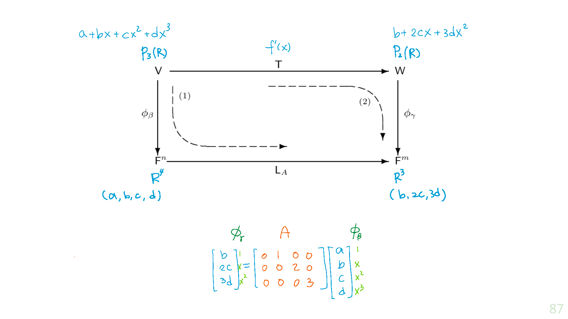
Let $\mathsf{V}$ and $\mathsf{W}$ be vector spaces of dimension $n$ and $m$, respectively, and let $\mathsf{T}:\mathsf{V}\to \mathsf{W}$ be a linear transformation. Define $A=[\mathsf{T}{]}_{\beta }^{\gamma }$, where $\beta$ and $\gamma$ are arbitrary ordered bases of $\mathsf{V}$ and $\mathsf{W}$, respectively. We are now able to use ${\varphi }_{\beta }$ and ${\varphi }_{\gamma }$ to study the relationship between the linear transformations $\mathsf{T}$ and ${\mathsf{L}}_A:{\mathsf{F}}^n\to {\mathsf{F}}^m$.

Consider the following two composites of linear transformations that map $\mathsf{V}$ into ${\mathsf{F}}^m$:

1. Map $\mathsf{V}$ into ${\mathsf{F}}^n$ with ${\varphi }_{\beta }$ and follow this transformation with ${\mathsf{L}}_A$; this yields the composite ${\mathsf{L}}_A{\varphi }_{\beta }$.

2. Map $\mathsf{V}$ into $\mathsf{W}$ with $\mathsf{T}$ and follow it by ${\varphi }_{\gamma }$ to obtain the composite ${\varphi }_{\gamma }\mathsf{T}$.

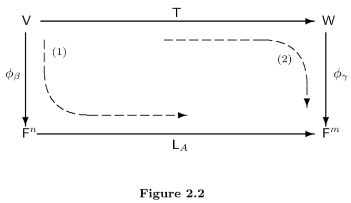
These 2 composites are depictedby the dashed arrows in the diagram. By a simple reformulation of Theorem 2.14, we may conclude that

$${\mathsf{L}}_A{\varphi }_{\beta }={\varphi }_{\gamma }\mathsf{T}$$

($[\mathsf{T}(u){]}_{\gamma }=[\mathsf{T}][u{]}_{\beta }$)

That is, the diagram "commutes." Heuristically, this relationship indicates that after $\mathsf{V}$ and $\mathsf{W}$ are identified with ${\mathsf{F}}^n$ and ${\mathsf{F}}^m$ via ${\varphi }_{\beta }$ and ${\varphi }_{\gamma }$, respectively, we may "identify" $\mathsf{T}$ with ${\mathsf{L}}_A$. This diagram allows us to transfer operations on abstract vector spaces to ones on ${\mathsf{F}}^n$ and ${\mathsf{F}}^m$.

Example 2.4.7

Recall the linear transformation $\mathsf{T}:{\mathsf{P}}_3(\mathbb{R})\to {\mathsf{P}}_2(\mathbb{R})$ defined by $\mathsf{T}(f(x))=f^{\prime }(x)$. Let $\beta$ and $\gamma$ be the standard ordered bases for ${\mathsf{P}}_3(\mathbb{R})$ and ${\mathsf{P}}_2(\mathbb{R})$, respectively, and let ${\varphi }_{\beta }:{\mathsf{P}}_3(\mathbb{R})\to {\mathbb{R}}^4$ and ${\varphi }_{\gamma }:{\mathsf{P}}_2(\mathbb{R})\to {\mathbb{R}}^3$ be the corresponding standard representations.

If $A=[\mathsf{T}]$, then

$$A=\left(\begin{array}{cccc}0& 1& 0& 0\\ 0& 0& 2& 0\\ 0& 0& 0& 3\end{array}\right)$$

Consider the polynomial $p(x)=2+x-3x^2+5x^3$. We show that

$${\mathsf{L}}_A{\varphi }_{\beta }(p(x))=\left(\begin{array}{cccc}0& 1& 0& 0\\ 0& 0& 2& 0\\ 0& 0& 0& 3\end{array}\right)\left(\begin{array}{c}2\\ 1\\ -3\\ 5\end{array}\right)=\left(\begin{array}{c}1\\ -6\\ 15\end{array}\right)$$

But since $\mathsf{T}(p(x))=p^{\prime }(x)=1-6x+15x^2$, we have

$${\varphi }_{\gamma }\mathsf{T}(p(x))=\left(\begin{array}{c}1\\ -6\\ 15\end{array}\right)$$

So

$${\mathsf{L}}_A{\varphi }_{\beta }(p(x))={\varphi }_{\gamma }\mathsf{T}(p(x))$$

2.5 The Change of Coordinate Matrix

Theorem 2.22

Let $\beta$ and ${\beta }^{\prime }$ be two ordered bases for a finite-dimensional vector space $\mathsf{V}$, and let $Q=[{\mathsf{I}}_{\mathsf{V}}{]}_{\beta }^{{\beta }^{\prime }}$. Then

• $Q$ is invertible.
• For any $v\in \mathsf{V},[v{]}_{\beta }=Q[v{]}_{{\beta }^{\prime }}$

The matrix $Q=[{\mathsf{I}}_{\mathsf{V}}{]}_{\beta }^{{\beta }^{\prime }}$ is called a change of coordinate matrix. Because of part (b) of the theorem, we say that $Q$ changes ${\beta }^{\prime }$-coordinates into $\beta$-coordinates. Observe that if $\beta =x_1,x_2,...,x_n$ and ${\beta }^{\prime }=x_1^{\prime },x_2^{\prime },...,x_n^{\prime }$, then

$$x_j^{\prime }=\sum _{i=1}^n{Q}_{ij}{x}_i$$

for $j=1,2,\cdots ,n$; that is, the jth column of $Q$ is $[x_j^{\prime }{]}_{\beta }$.

Example 2.5.1

In ${\mathbb{R}}^2$, and let

$$\beta =\{(1,1),(1,-1)\},{\beta }^{\prime }=\{(2,4),(3,1)\}$$

Since

$$(2,4)=3(1,1)-1(1,-1),(3,1)=2(1,1)+1(1,-1)$$

the change of coordinate matrix $Q$ changing ${\beta }^{\prime }$-coordinates into $\beta$-coordinates is

$$Q=\left(\begin{array}{cc}3& 2\\ -1& 1\end{array}\right)$$

For instance,

$$[(2,4){]}_{\beta }=Q[(2,4){]}_{{\beta }^{\prime }}=Q\left(\begin{array}{c}1\\ 0\end{array}\right)=\left(\begin{array}{c}3\\ -1\end{array}\right)$$

For the remainder of this section, we consider only linear transformations that map a vector space $\mathsf{V}$ into itself. Such a linear transformation is called a linear operator on $\mathsf{V}$

Theorem 2.23

Let $\mathsf{T}$ be a linear operator on a finite-dimensional vector space $\mathsf{V}$, and let $\beta$ and ${\beta }^{\prime }$ be ordered bases for $\mathsf{V}$. Suppose $Q$ is the change of coordinate matrix that changes ${\beta }^{\prime }$-coordinates into $\beta$-coordinates. Then

$$[\mathsf{T}{]}_{{\beta }^{\prime }}=Q^{-1}[\mathsf{T}{]}_{\beta }Q$$

Proof:

$$Q[\mathsf{T}{]}_{{\beta }^{\prime }}=[\mathsf{I}{]}_{{\beta }^{\prime }}^{\beta }=[\mathsf{T}{]}_{{\beta }^{\prime }}^{{\beta }^{\prime }}=[\mathsf{IT}{]}_{{\beta }^{\prime }}^{\beta }=[\mathsf{TI}{]}_{{\beta }^{\prime }}^{\beta }=[\mathsf{T}{]}_{\beta }^{\beta }[\mathsf{I}{]}_{{\beta }^{\prime }}^{\beta }=[\mathsf{I}{]}_{\beta }Q.$$

Example 2.5.2: Calculation about coordination change

Let $\mathsf{T}$ be the linear operator on ${\mathbb{R}}^2$ defined by

$$\mathsf{T}\left(\begin{array}{c}a\\ b\end{array}\right)=\left(\begin{array}{c}3a-b\\ a+3b\end{array}\right)$$

Let

$$\beta =\{(1,1),(1,-1)\},{\beta }^{\prime }=\{(2,4),(3,1)\}$$

be the ordered bases. It can be known that

$$[\mathsf{T}{]}_{\beta }=\left(\begin{array}{cc}3& 1\\ -1& 3\end{array}\right)$$

(Here gives details about the result above)

Given that $[\mathsf{T}{]}_{\beta }=Q^{\prime -1}[\mathsf{T}{]}_{\gamma }{Q}^{\prime }$, where $\gamma$ is standard ordered basis, thus

$$[\mathsf{T}{]}_{\gamma }=\left(\begin{array}{cc}3& -1\\ 1& 3\end{array}\right)$$

And

$$Q^{\prime }=\left(\begin{array}{cc}1& 1\\ 1& -1\end{array}\right),Q^{\prime -1}=\frac{1}{2}\left(\begin{array}{cc}1& 1\\ 1& -1\end{array}\right).$$

So

$$\begin{array}{rlr}{}_{\beta }& =\frac{1}{2}\left(\begin{array}{cc}1& 1\\ 1& -1\end{array}\right)\left(\begin{array}{cc}3& -1\\ 1& 3\end{array}\right)\left(\begin{array}{cc}1& 1\\ 1& -1\end{array}\right)& =\left(\begin{array}{cc}3& 1\\ -1& 3\end{array}\right)\end{array}$$

The change of coordinate matrix that changes ${\beta }^{\prime }$-coordinate into $\beta$-coordinate is

$$Q=\left(\begin{array}{cc}3& 2\\ -1& 1\end{array}\right)$$

and

$$Q^{-1}=\frac{1}{5}\left(\begin{array}{cc}1& -2\\ 1& 3\end{array}\right)$$

hence, by theorem 2.23:

$$[\mathsf{T}{]}_{{\beta }^{\prime }}=Q^{-1}[\mathsf{T}{]}_{\beta }Q=\left(\begin{array}{cc}4& 1\\ -2& 2\end{array}\right)$$

To show that this's the correct matrix, we can verify that the image under $\mathsf{T}$ of each vector of ${\beta }^{\prime }$ is the linear combination of the vectors of ${\beta }^{\prime }$ with the entries of thecorresponding column as its coefficients. For example, the image of the 2nd vector in ${\beta }^{\prime }$ is

$$\mathsf{T}\left(\begin{array}{c}3\\ 1\end{array}\right)=\left(\begin{array}{c}8\\ 6\end{array}\right)=1\left(\begin{array}{c}2\\ 4\end{array}\right)+2\left(\begin{array}{c}3\\ 1\end{array}\right)$$

Note that the coeffficients of the linear combination are the entries of the 2nd column of $[\mathsf{T}{]}_{{\beta }^{\prime }}$

Example 2.5.3： Application about coordination change

Recall the reflection about the x-axis in Example 3 in Section 2.1. The rule $(x,y)\to (x,-y)$ is easy to obtain. Let $\mathsf{T}$ be the reflection about the line $y=2x$. We wish to find an expression for $\mathsf{T}(a,b)$ for any $(a,b)\in {\mathbb{R}}^2$. Since $\mathsf{T}$ is linear, it is determined by its values on a basis for ${\mathbb{R}}^2$. For basis vectors,

$$\mathsf{T}(1,2)=(1,2),\mathsf{T}(-2,1)=(2,-1)$$

Therefore if we let

$${\beta }^{\prime }=\{\left(\begin{array}{c}1\\ 2\end{array}\right),\left(\begin{array}{c}-2\\ 1\end{array}\right)\}$$

Then the matrix representing $\mathsf{T}$ in the basis ${\beta }^{\prime }=\{(1,2),(-2,1)\}$ is

$$[\mathsf{T}{]}_{{\beta }^{\prime }}=\left(\begin{array}{cc}1& 0\\ 0& -1\end{array}\right)$$

Let $\beta$ be the standard ordered basis for ${\mathbb{R}}^2$, and let $Q$ be the matrix that changes ${\beta }^{\prime }$-coordinates into $\beta$-coordinates. Then

$$Q=\left(\begin{array}{cc}1& -2\\ 2& 1\end{array}\right)$$

and $Q^{-1}[\mathsf{T}{]}_{\beta }Q=[\mathsf{T}{]}_{{\beta }^{\prime }}$. We can solve this equation for $[\mathsf{T}{]}_{\beta }$ to obtain that $[\mathsf{T}{]}_{\beta }=Q[\mathsf{T}{]}_{{\beta }^{\prime }}{Q}^{-1}$. Because

$$Q^{-1}=\frac{1}{5}\left(\begin{array}{cc}1& 2\\ -2& 1\end{array}\right)$$

Then it can be verified that

$$[\mathsf{T}{]}_{\beta }=\frac{1}{5}\left(\begin{array}{cc}-3& 4\\ 4& 3\end{array}\right)$$

Since $\beta$ is the standard ordered basis, it follows that $\mathsf{T}$ is left-multiplication by $[\mathsf{T}{]}_{\beta }$. Thus for any $(a,b)\in {\mathbb{R}}^2$, we have

$$\mathsf{T}\left(\begin{array}{c}a\\ b\end{array}\right)=\frac{1}{5}\left(\begin{array}{cc}-3& 4\\ 4& 3\end{array}\right)\left(\begin{array}{c}a\\ b\end{array}\right)=\frac{1}{5}\left(\begin{array}{c}-3a+4b\\ 4a+3b\end{array}\right)$$

Corollary

Let $A\in {\mathsf{M}}_{n\times n}(F)$, and let $\gamma$ be an ordered basis for ${\mathsf{F}}^n$. Then

$$[{\mathsf{L}}_A{]}_{\gamma }=Q^{-1}AQ$$

where $Q$ is the $$\begin{gathered} n \\ timesn \end{gathered}$$ matrix whose jth column is the jth vector of $\gamma$.

Example 2.5.4

Let

$$A=\left(\begin{array}{ccc}2& 1& 0\\ 1& 1& 3\\ 0& -1& 0\end{array}\right)$$

and let

$$\gamma =\{\left(\begin{array}{c}-1\\ 0\\ 0\end{array}\right),\left(\begin{array}{c}2\\ 1\\ 0\end{array}\right),\left(\begin{array}{c}1\\ 1\\ 1\end{array}\right)\}$$

which is an ordered basis for ${\mathbb{R}}^3$. Let $Q$ be the $3\times 3$ matrix whose jth column is the jth vector of $\gamma$. Then

$$Q=\left(\begin{array}{ccc}-1& 2& 1\\ 0& 1& 1\\ 0& 0& 1\end{array}\right)\text{ and }{Q}^{-1}=\left(\begin{array}{ccc}-1& 2& -1\\ 0& 1& -1\\ 0& 0& 1\end{array}\right)$$

So by the preceding corollary,

$$[{\mathsf{L}}_A{]}_{\gamma }=Q^{-1}AQ=\left(\begin{array}{ccc}0& 2& 8\\ -1& 4& 6\\ 0& -1& -1\end{array}\right)$$

Definition

Let $A,B$ be matrices in ${\mathsf{M}}_{n\times n}(F)$. We say $B$ is similar to $A$ if there exists an invertible matrix $Q$ such that

$$B=Q^{-1}AQ$$