7 Direct Approaches to Continuous Optimal Control

Come from Chapter 13 in Numerical Optimal Control by Moritz Diehl and Sebastien Gros

Direct methods to continuous optimal control finitely parameterize the infinite dimensional decision variables, notably the controls $\mathit{\alpha }(t)$, s.t. the original problem is approximated by a finite dimensional nonlinear program (NLP). This NLP can then be addressed by structure exploiting numerical NLP solution methods. For this reason, the approach is often characterized as “First discretize, then optimize.”

The direct approach connects easily to all optimization methods developed in the continuous optimization community. Most successful direct methods even parameterize the problem such that the resulting NLP has the structure of a discrete time optimal control problem, such that all the techniques and structures about dynamic programming are applicable. For this reason, the current chapter is kept relatively short; its major aim is to outline the major concepts and vocabulary in the field.

We start by describing direct single shooting, direct multiple shooting, and direct collocation and a variant pseudospectral methods. We also discuss how sensitivities are computed in the context of shooting methods. The optimization problem formulation we address in this chapter typically read as (but are not limited to):

$$\begin{array}{rl}\underset{{\mathit{x}}_0,{\mathit{\alpha }}_0,{\mathit{x}}_1,\dots ,{\mathit{\alpha }}_{N-1},{\mathit{x}}_N}{min}& {\int }_0^{T}r(\mathit{x}(t),\mathit{\alpha }(t))\mathrm{d}t+g(\mathit{x}(T))\\ \text{ subject to }& \mathit{x}(0)-x^0=0,& & (\text{initial value})\\ & \dot{\mathit{x}}(t)-\mathit{f}(\mathit{x}(t),\mathit{\alpha }(t))=0,& & (\text{system dynamics})\\ & \mathit{s}(\mathit{x}(t),\mathit{\alpha }(t))\le 0,& & (\text{path constraints})\\ & \mathit{b}(\mathit{x}(T))\le 0.& & (\text{terminal constraints})\end{array}$$

For many optimal control problems (OCPs), the system state derivatives $\dot{\mathit{x}}(t)$ are provided via an implicit function, or even via a Differential-Algebraic Equation (DAE). The methods presented hereafter are applicable to all these cases with some minor modifications. The direct methods differ in how they transcribe this problem into a finite NLP. The optimal control problem above has a fixed initial value, which simplifies in particular the single shooting method, but all concepts can in a straightforward way be generalized to other OCP formulations with free initial values.

7.1 Direct Single Shooting

All shooting methods use an embedded ODE or differential algebraic equations (DAE) solver in order to eliminate the continuous time dynamic system. They do so by first parameterizing the control function $\mathit{\alpha }(t)$, e.g. by polynomials, by piecewise constant functions, or, more generally, by piecewise polynomials. We denote the finite control parameters by the vector $\mathit{q}$, and the resulting control function by $\mathit{\alpha }(t,\mathit{q})$.

The most widespread parameterization are piecewise constant controls, for which we choose a fixed time grid $0=t_0<t_1<\dots <t_N=T$, and $N$ parameters ${\mathit{q}}_i\in {\mathbb{R}}^{n_{\alpha }},i=0,\dots ,N-1$, and then we set

$$\mathit{\alpha }(t,\mathit{q})={\mathit{q}}_k\text{ for }t\in [t_k,t_{k+1}].$$

Thus, the dimension of the vector $\mathit{q}=({\mathit{q}}_0,\dots ,{\mathit{q}}_{N-1})$ is of dimension $N{n}_u$.

Single shooting is a sequential approach that calculate OCP recursively. In single shooting, we regard the states $\mathit{x}(t)$ on $[0,T]$ as dependent variables that are obtained by a forward integration of the dynamic system, starting at ${\mathit{x}}^0$ and using the controls input $\mathit{\alpha }(t,\mathit{q})$. We denote the resulting trajectory as $\mathit{x}(t,\mathit{q})$.

In order to discretize inequality path constraints, we choose a grid, typically the same as for the control discretization, at which we check the inequalities. Thus, in single shooting, we transcribe the optimal control problem into the following NLP, that is visualized in Figure 13.1.

$$\begin{array}{rl}\underset{\mathit{q}\in {\mathbb{R}}^{N{n}_u}}{\min }& {\int }_0^{T}r(\mathit{x}(t,\mathit{q}),\mathit{\alpha }(t,\mathit{q}))\mathrm{d}t+g(\mathit{x}(T,\mathit{q}))\\ \text{ subject to }& \mathit{s}(\mathit{x}(t_i,\mathit{q}),\mathit{u}(t_i,\mathit{q}))\le 0,i=0,\dots ,N-1& & (\text{path constraints})\\ & \mathit{b}(\mathit{x}(T,\mathit{q}))\le 0.& & \text{(terminal constraints)}\end{array}$$

NLP structure in single shooting

As the only variable of this NLP is the vector $\mathit{q}\in {\mathbb{R}}^{N{n}_{\alpha }}$ that influences nearly all problem functions, the above problem can usually be solved by a dense NLP solver in a black-box fashion. As the problem functions and their derivatives are expensive to compute, while a small quadratic programming (QP) is cheap to solve, often Sequential Quadratic Programming (SQP) is used, e.g. the codes NPSOL or SNOPT. Let us first assume the Hessian needs not be computed but can be obtained e.g. by Broyden-Fletcher-Goldfarb-Shanno (BFGS) updates.

The computation of the derivatives can be done in different ways with a different complexity:

first, we can use forward derivatives, using finite differences or algorithmic differentiation. Taking the computational cost of integrating one time interval as one computational unit, this means that one complete forward integration costs $N$ units. Given that the vector $\mathit{q}$ has $N{n}_{\alpha }$ components, this means that the computation of all derivatives costs $(N{n}_{\alpha }+1)N$ units when implemented in the most straightforward way. This number can still be reduced by one half if we take into account that controls at the end of the horizon do not influence the first part of the trajectory. We might call this way the reduced derivative computation as it computes directly only the reduced quantities needed in each reduced QP.

Second, if the number of output quantities such as objective and inequality constraints is not big, we can use the principle of reverse automatic differentiation in order to generate the derivatives. In the extreme case that no inequality constraints are present and we only need the gradient of the objective, this gradient can cheaply be computed by reverse Algorithmic Differentiation (AD), as done in the so called gradient methods. Note that in this case the same adjoint differential equations of the indirect approach can be used for reverse computation of the gradient, but that in contrast to the indirect method we do not eliminate the controls, and we integrate the adjoint equations backwards in time. The complexity for one gradient computation is only $4N$ computational units. However, each additional state constraint necessitates a further backward sweep.

Third, in the case that we have chosen piecewise controls, as here, we might use the fact that after the piecewise control discretization we have basically transformed the continuous time OCP into a discrete time OCP (see next section). Then we can compute the derivatives with respect to both ${\mathit{x}}_i$ and ${\mathit{q}}_i$ on each interval separately, which costs $(n_x+n_{\alpha }+1)$ units. This means a total derivative computation cost of $N(n_x+n_{\alpha }+1)$ units. In contrast to the second (adjoint) approach, this approach can handle an arbitrary number of path inequality constraints, like the first one. Note that it has the same complexity that we obtain in the standard implementation of the multiple shooting approach, as explained next. We remark here already that both shooting methods can each implement all the above ways of derivative generation, but differ in one respect only, namely that single shooting is a sequential and multiple shooting a simultaneous(calculates all states and controls at the same time) approach.

Example 7.1

OCP formulation

Let us illustrate the single shooting method using the following simple OCP:

$$\begin{array}{}\text{(13.1)}& \begin{array}{rlr}\underset{\mathit{x}(.),\mathit{\alpha }(.)}{\min }& {\int }_0^5{x}_1(t{)}^2+10x_2(t{)}^2+\alpha (t{)}^2\mathrm{d}t& \\ \text{ subject to }& {\dot{x}}_1(t)=x_1(t)x_2(t)+\alpha (t),& & x_1(0)=0\\ & {\dot{x}}_2(t)=x_1(t),& & x_2(0)=1,\\ & \alpha (t)\ge -1,x_1(t)\ge -0.6,& & t\in [0,T],\end{array}\end{array}$$

The resulting solution is illustrated in Figure 13.1, together with the sparsity patterns of the Jacobian of the inequality constraint function, i.e.

$$\frac{\partial }{\partial \mathit{q}}s(x(t_i,\mathit{q}),u(t_i,\mathit{q})),$$

and the one of the Hessian of the Lagrange function.

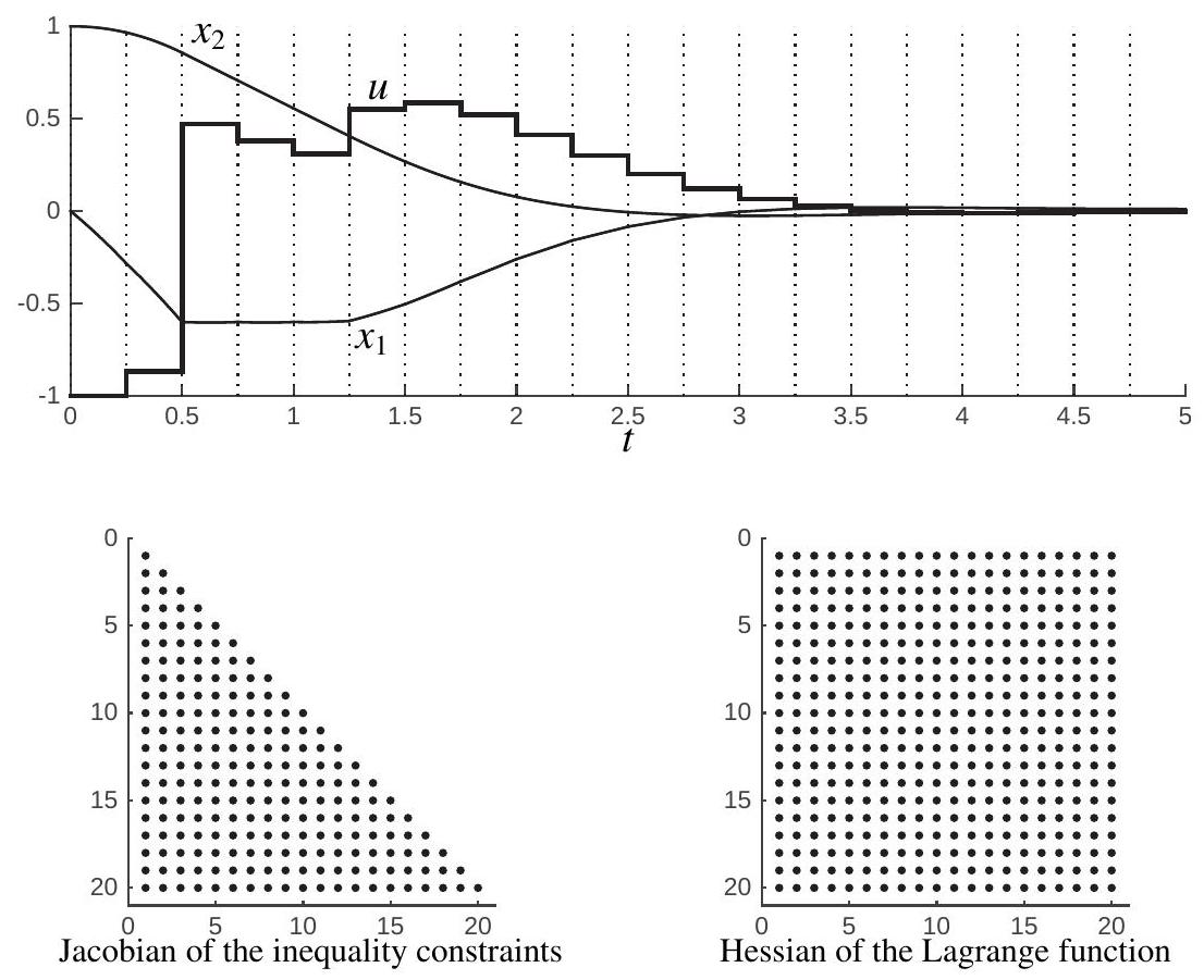
Figure 13.1: Solution to OCP (13.1) using a discretization based on single shooting, with $N=20$ and using a $4$-steps Runge-Kutta integrator of order $4$. The upper graph reports the states and input trajectories. The lower graphs report the sparsity pattern of the Jacobian of the inequality constraints in the resulting NLP and the sparsity pattern of the Hessian of the Lagrange function.

Nonlinearity propagation in direct single shooting

Unfortunately, direct single shooting often suffers from ill-conditioned problem. More specifically, when deploying single shooting in the context of direct optimal control a difficulty can arise from the nonlinearity of the "simulation" function $\mathit{x}(t,\mathit{q})$ with respect to the control inputs $\mathit{q}$ for a large simulation time $t$. We illustrate this problem using the following example:

$$\begin{array}{}\text{(13.2a)}& & {\dot{x}}_1=10(x_2-x_1)\text{(13.2b)}& & {\dot{x}}_2=x_1(q-x_3)-x_2\text{(13.2c)}& & {\dot{x}}_3=x_1{x}_2-3x_3\end{array}$$

where $\mathit{x}=(x_1,x_2,x_3)\in {\mathbb{R}}^3$ and $q\in \mathbb{R}$ is a constant control input. Note that the nonlinearities in this ODE result from apparently innocuous bilinear expressions. We are then interested in the relationship $q\to \mathit{x}(t,q)$ for different values of $t$. The initial conditions of the simulation were selected as $\mathit{x}(t){|}_{t=0}=(0,0,0)$ and $q\in [18,38]$. The resulting relationship is displayed in Fig. 13.2. One can observe that while the relationship is not very nonlinear for small integration times $t$, it becomes extremely nonlinear for large times $t$, even though the ODE under consideration here appears simple and mildly nonlinear.

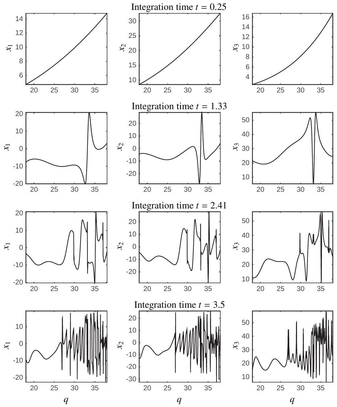
Figure 13.2: Illustration of the propagation of nonlinearities in the simple dynamic system (13.2). One can observe that for a short integration time $t=0.25$ (first row), the relationship $q\to \mathit{x}(t,q)$ is close to linear. However, as the integration time increases to $t=1.33,2.41,3.5$, the relationship $q\to \mathit{x}(t,q)$ becomes extremely nonlinear. While the effect of integration time is not necessarily as dramatic as for this specific example, large integration times yield strong nonlinear relationship $q\to \mathit{x}(t,q)$ for many nonlinear dynamics.

This example ought to warn the reader that the function $\mathit{x}(t,\mathit{q})$ resulting from the simulation of nonlinear dynamics can be extremely nonlinear. As a result, functions such as the constraints and cost function in the NLP resulting form the discretization of an optimal control problem via single-shooting can be themselves extremely nonlinear functions of the input sequence $\mathit{q}$. Because most NLP solvers proceed to find a candidate solution via taking successive linearization of the KKT conditions of the problem at hand, the presence of very nonlinear functions in the NLP problem typically invalidates these approximations outside of a very small neighborhood of the linearization point.

These observations entails that in practice, when using single-shooting, a very good initial guess for $\mathit{q}$ is often required. For many problems, such an initial guess is very difficult to construct. As in the context of indirect methods, these observations motivate the use of alternative transcription techniques.

7.2 Direct Multiple Shooting

The direct multiple shooting method was originally developed by Bock and Plitt. It follows similar ideas as the indirect multiple-shooting approach, but recast in the direct optimization framework, where the input profile is also discretized and part of the decision variables.

The idea behind the direct multiple-shooting approach stems from the observation that performing long integration of dynamics can be counterproductive for discretizing continuous optimal control problems into NLPs, and tackles the problem by limiting the integration over arbitrarily short time intervals. Direct multiple-shooting performs first a finite-dimensional discretization of the continuous control input $\mathit{\alpha }(t)$, most commonly using a piecewise control discretization on a chosen time grid, exacly as we did in single shooting, i.e. we set

$$\mathit{\alpha }(t)={\mathit{q}}_i\text{ for }t\in [t_i,t_{i+1}]$$

In contrast to single shooting, it then solves the ODE separately on each interval $[t_i,t_{i+1}]$, starting with artificial initial values ${\mathit{\beta }}_i$ :

$$\begin{array}{rl}{\dot{\mathit{x}}}_i(t,{\mathit{\beta }}_i,{\mathit{q}}_i)& =\mathit{f}({\mathit{x}}_i(t,{\mathit{\beta }}_i,{\mathit{q}}_i),{\mathit{q}}_i),t\in [t_i,t_{i+1}],\\ {\mathit{x}}_i(t_i,{\mathit{\beta }}_i,{\mathit{q}}_i)& ={\mathit{\beta }}_i.\end{array}$$

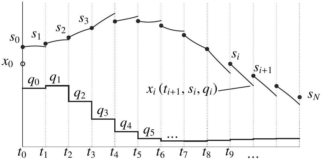
Figure 13.3: Illustration of the direct multiple shooting method. A piecewiseconstant input profile parametrized by ${\mathit{q}}_{0,\dots ,N-1}$ is deployed on the time grid $t_{0,\dots ,N}$. The discrete states ${\mathit{\beta }}_{0,\dots ,N}$ act as "checkpoints" on the continuous state trajectories $\mathit{x}(t)$ at all discrete time points $t_{0,\dots ,N}$. Numerical integrators build the simulations ${\mathit{x}}_i(t,{\mathit{\beta }}_i,{\mathit{q}}_i)$ over each time interval $[t_i,t_{i+1}]$. The state trajectory held in the NLP solver becomes continuous only when the solution of the NLP is reached, where the continuity conditions ${\mathit{x}}_i(t_{i+1},{\mathit{\beta }}_i,{\mathit{q}}_i)-{\mathit{\beta }}_{i+1}$ are enforced.

See Figure 13.3 for an illustration. Thus, we obtain trajectory pieces ${\mathit{x}}_i(t,{\mathit{\beta }}_i,{\mathit{q}}_i)$. Likewise, we numerically compute the integrals

$$l_i({\mathit{\beta }}_i,{\mathit{q}}_i):={\int }_{t_i}^{t_{i+1}}r({\mathit{x}}_i(t,{\mathit{\beta }}_i,{\mathit{q}}_i),{\mathit{q}}_i)\mathrm{d}t.$$

The problem of piecing the trajectories together, i.e. ensuring the continuity condition ${\mathit{\beta }}_{i+1}={\mathit{x}}_i(t_{i+1},{\mathit{\beta }}_i,{\mathit{q}}_i)$ is left to the NLP solver.

Finally, we choose a time grid on which the inequality path constraints are checked. It is common to choose the same time grid as for the discretization of the controls as piecewise constant, such that the constraints are checked based on the artificial initial values ${\mathit{\beta }}_i$. However, a much finer sampling is possible as well, provided that the numerical integrator building the simulations over the various time intervals $[t_k,t_{k+1}]$ report not only their final state ${\mathit{x}}_i(t_{i+1},{\mathit{\beta }}_i,{\mathit{q}}_i)$, but also intermediate values. An integrator reporting the state (or some function of the state) over a refined or arbitrary time grid is sometimes labelled as continuous-output integrator.

The NLP arising from a discretization of an OCP based on multiple shooting typically reads as:

$$\begin{array}{rl}\underset{\mathit{S},\mathit{q}}{\min }& \sum _{i=0}^{N-1}{l}_i({\mathit{\beta }}_i,{\mathit{q}}_i)+g\left({\mathit{\beta }}_N\right)\\ \text{ subject to }& {\mathit{x}}_0-{\mathit{\beta }}_0=0,& & & & \text{ (initial value)}\\ & {\mathit{x}}_i(t_{i+1},{\mathit{\beta }}_i,{\mathit{q}}_i)-{\mathit{\beta }}_{i+1}=0,& & i=0,\dots ,N-1& & \text{(continuity)}\\ & h({\mathit{\beta }}_i,{\mathit{q}}_i)\le 0,& & i=0,\dots ,N& & \text{ (path constraints)}\\ & r\left({\mathit{\beta }}_N\right)\le 0.& & & & \text{ (terminal constraints)}\end{array}$$

It is visualized in Figure 13.3. Let us illustrate the multiple shooting method using the OCP $(13.1)$. Here the ordering of the equality constraints and variables is important in order to get structured sparsity patterns. In this example, the variables are ordered in time as:

$${\mathit{\beta }}_{1,0},{\mathit{\beta }}_{2,0},{\mathit{q}}_0,{\mathit{\beta }}_{1,1},{\mathit{\beta }}_{2,1},{\mathit{q}}_1,\dots ,{\mathit{q}}_{N-1},{\mathit{\beta }}_{1,N},{\mathit{\beta }}_{2,N}$$

and the constraints are also ordered in time. The resulting solution is illustrated in Figure 13.4, together with the sparsity patterns of the Jacobian of the equality constraint function, and the one of the Hessian of the Lagrange function.

Most important, the sparsity structure arising from a discretization based on multipleshooting (see Figure 13.4 for an illustration) ought to be exploited in the NLP solver.

Example 13.2

Let us tackle the OCP (13.1) of Example 13.1 via direct multipleshooting. A 4-step RK4 integrator has been used here, deployed on $N=20$ shooting intervals. The variables have been ordered as:

$${\mathit{\beta }}_0,{\mathit{q}}_0,{\mathit{\beta }}_1,{\mathit{q}}_1,\dots ,{\mathit{\beta }}_{N-1},{\mathit{\alpha }}_{N-1},{\mathit{\beta }}_N$$

and the shooting constraints are also imposed time-wise.

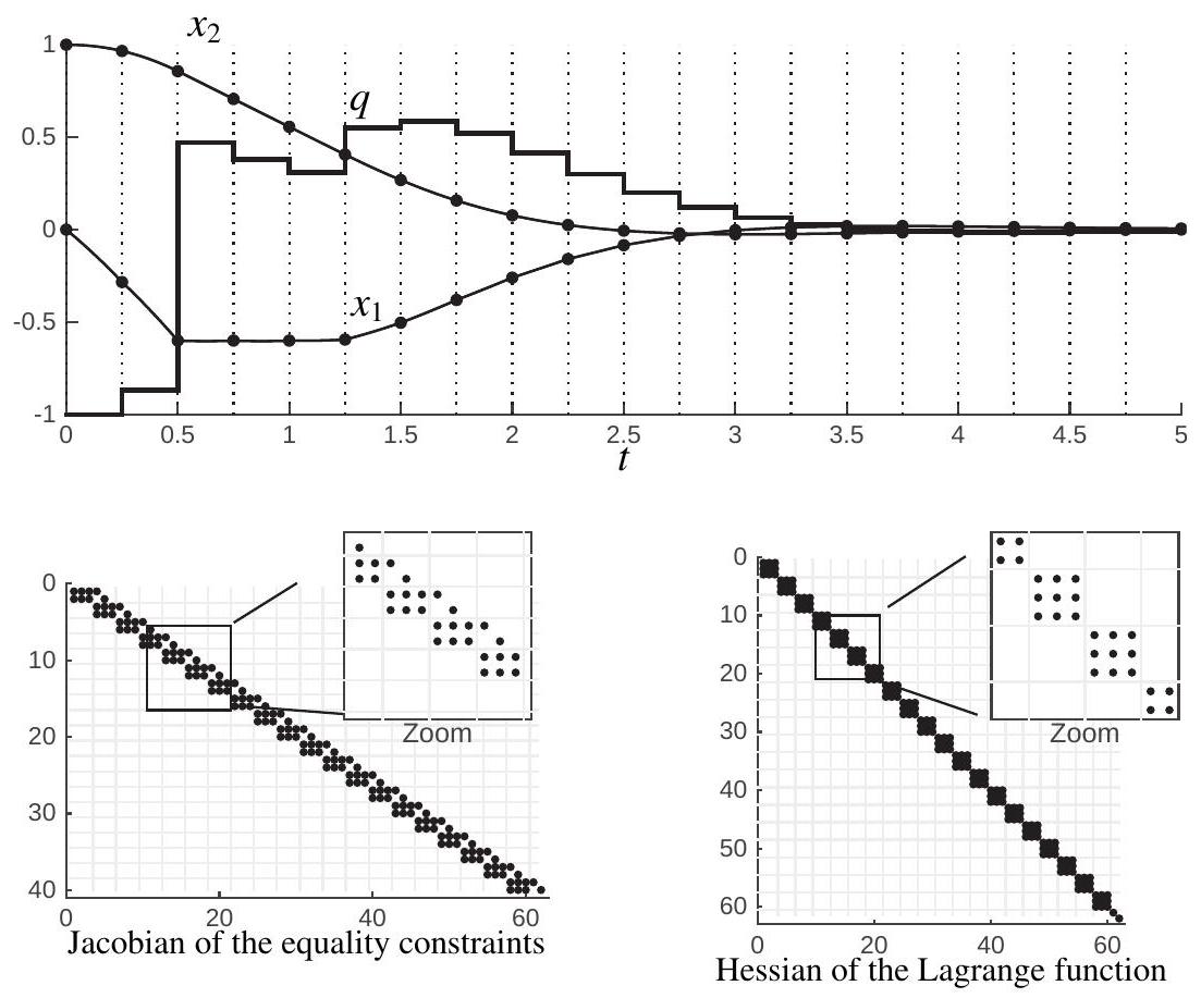
Figure 13.4: Solution to OCP $(13.1)$ using a discretization based on multiple shooting, with $N=20$ and using a 4-steps Runge-Kutta integrator of order 4. The upper graph reports the states and input trajectories at the solution, where the continuity condition holds. The lower graphs report the sparsity pattern of the Jacobian of the equality constraints in the resulting NLP and the sparsity pattern of the Hessian of the Lagrange function. The Hessian of the Lagrange function arising from multiple-shooting is block-diagonal, due to the separability of the Lagrange function. The Jacobian of the inequality constraints is diagonal in this example, and block-diagonal in general.

The resulting solution is displayed in Figure 13.4, where one can observe the discrete state trajectories (black dots) at the discrete time instants $t_{0,\dots ,N}$ together with the simulations delivered by the integrators at the solution. One can also observe the very specific sparsity patterns of the Jacobian of the equality constraints and of the Hessian of the Lagrange function that arise from the direct multiple-shooting approach.

Remark on Schlöder's Reduction Trick

We point out here that the derivatives of the condensed QP could also directly be computed, using the reduced way, as explained as first variant in the context of single shooting. It exploits the fact that the initial value ${\mathit{x}}_0$ is fixed in the nonlinear model predictive control (NMPC) problem, changing the complexity of the derivative computations. It is only advantageous for large state but small control dimensions as it has a complexity of $N^2{n}_{\alpha }$. It was originally developed by Schlöder in the context of Gauss-Newton methods and generalized to general SQP shooting methods. A further generalization of this approach to solve a "lifted" (larger, but equivalent) system with the same computational cost per iteration is the so called lifted Newton method where also an analysis of the benefits of lifting is made.

The main advantages of lifted Newton approaches such as multiple shooting compared with single shooting are the facts that

• we can also initialize the state trajectory,
• they show superior local convergence properties in particular for unstable systems. An interesting remark is that if the original system is linear, continuity is perfectly satisfied in all SQP iterations, and single and multiple shooting would be identical. Also, it is interesting to recall that the Lagrange multipliers ${\lambda }_i$ for the continuity conditions are an approximation of the adjoint variables, and that they indicate the costs of continuity.

Finally, it is interesting to note that a direct multiple shooting algorithm can be made a single shooting algorithm easily: we only have to overwrite, before the derivative computation, the states $\mathit{\beta }$ by the result of a forward simulation using the controls $\mathit{q}$ obtained in the last Newton-type iteration. From this perspective, we can regard single shooting as a variant of multiple shooting where we perturb the result of each iteration by a "feasibility improvement" that makes all continuity conditions feasible by the forward simulation, implicitly giving priority to the control guess over the state guess.

7.3 Direct Collocation method

A third important class of direct methods are the so-called direct transcription methods, most notably direct collocation. The discretization method applied here is directly inspired from the collocation-based simulation, and very similar to the indirect collocation method.

Here we discretize the infinite OCP in both controls and states on a fixed and relatively fine grid $t_k$, with $k=0,\dots ,N$. We denote the discrete states on the grid points $t_k$ as ${\mathit{\beta }}_k$. We choose a parameterization of the controls on the same grid typically as piecewise constant, with control parameters ${\mathit{q}}_k$, which yields on each interval $[t_k,t_{k+1}]$ a constant control $\mathit{\alpha }(t)={\mathit{q}}_k$.

On each collocation interval $[t_k,t_{k+1}]$ a set of $d$ collocation times $t_{k,i}\in [t_k,t_{k+1}]$ is chosen, with $i=0,\dots ,d$. The trajectory of each state on the time interval $[t_k,t_{k+1}]$ is approximated by a polynomial ${\mathit{p}}_k(t,{\mathit{v}}_k)\in {\mathbb{R}}^{n_x}$ having the coefficients ${\mathit{v}}_k\in {\mathbb{R}}^{n_x(d+1)}$.

The collocation-based integration of the state dynamics on a time interval $[t_k,t_{k+1}]$ starting from the initial value ${\mathit{\beta }}_k$ hinges on solving the collocation equation:

$$\begin{array}{}\text{(13.4)}& {\mathit{c}}_k({\mathit{v}}_k,{\mathit{\beta }}_k,{\mathit{q}}_k)=\left[\begin{array}{c}{\mathit{v}}_{k,0}-{\mathit{\beta }}_k\\ {\dot{\mathit{p}}}_k(t_{k,1},{\mathit{v}}_k)-\mathit{f}({\mathit{v}}_{k,1},t_{k,1},{\mathit{q}}_k)\\ ⋮\\ {\dot{\mathit{p}}}_k(t_{k,d},{\mathit{v}}_k)-\mathit{f}({\mathit{v}}_{k,d},t_{k,d},{\mathit{q}}_k)\end{array}\right]=0.\end{array}$$

for the variables ${\mathit{v}}_{k,i}\in {\mathbb{R}}^{n_x}$, with $i=0,\dots ,d$.

We now turn to building the NLP based on direct collocation. In addition to solving the collocation equations $(13.4)$ for $k=0,\dots ,N-1$, we also require continuity accross the interval boundaries, i.e. we require that

$${\mathit{p}}_k(t_{k+1},{\mathit{v}}_k)-{\mathit{\beta }}_{k+1}=0$$

holds for $k=0,\dots ,N$.

One finally ought to approximate the integrals ${\int }_{t_k}^{t_{k+1}}r(x,u)\mathrm{d}t$ on the collocation intervals by a quadrature formula using the same collocation points, which we denote by the a term $l_k({\mathit{v}}_k,{\mathit{\beta }}_k,{\mathit{q}}_k)$. Path constraints can be enforced on the fine time grid $t_{k,i}$, though it is common to enforce them only on the interval boundaries $t_k$ in order to reduce the amount of inequality constraints in the resulting NLP.

It is interesting to observe, that an arbitrary sampling of the state dynamics is possible by enforcing the path constraints at arbitrary time points $t$ via the interpolation $p_k(t,{\mathit{v}}_k)$. However, it is important to point out that the high integration order of collocation schemes holds only at the the main time grid $t_k$, such that interpolations at finer time grids, including the grid $t_{k,i}$, hold a lower numerical accuracy. In the following formulations, we will enforce the path constraints on the main time grid $t_k$.

Direct Collocation yields a large scale but sparse NLP, which can typically be written in the form

$$\begin{array}{rlr}\underset{\mathit{v},\mathit{\beta },\mathit{q}}{\min }& g\left({\mathit{\beta }}_N\right)+\sum _{k=0}^{N-1}{l}_k({\mathit{v}}_k,{\mathit{\beta }}_k,{\mathit{q}}_k)& \\ \text{ subject to }& {\mathit{\beta }}_0-{\mathit{x}}_0=0& & & & \text{(fixed initial value)}\\ & {\mathit{c}}_k({\mathit{v}}_k,{\mathit{\beta }}_k,{\mathit{q}}_k)=0,& & k=0,\dots ,N-1& & \text{ (collocation conditions)}\\ & {\mathit{p}}_k(t_{k+1},{\mathit{v}}_k)-{\mathit{\beta }}_{k+1}=0,& & k=0,\dots ,N-1& & \text{(continuity conditions)}\\ & \mathit{s}({\mathit{\beta }}_k,{\mathit{q}}_k)\le 0,& & k=0,\dots ,N-1,& & \text{ (path constraints), }\\ & \mathit{b}\left({\mathit{\beta }}_N\right)\le 0& & & & \text{ (terminal constraints). }\end{array}$$

One ought to observe that the discrete state variables ${\mathit{\beta }}_k$ or alternatively the collocation variables ${\mathit{v}}_{k,0}$ can be eliminated via the first linear equality in each collocation equations ${\mathit{c}}_k({\mathit{v}}_k,{\mathit{q}}_k,{\mathit{\beta }}_k)=0$. It is in fact common to formulate the NLP arising from direct collocation without the ${\mathit{\beta }}_k$ and enforcing continuity directly within the collocation equations. It then reads as follows:

$$\begin{array}{}\text{(13.5)}& \begin{array}{rl}\underset{\mathit{v},\mathit{q}}{\min }& g\left({\mathit{v}}_{N,0}\right)+\sum _{k=0}^{N-1}{l}_k({\mathit{v}}_k,{\mathit{q}}_k)\\ \text{ subject to }& {\mathit{v}}_{0,0}-{\mathit{x}}_0=0,\\ & {\dot{\mathit{p}}}_k(t_{k,i},{\mathit{v}}_k)-\mathit{f}({\mathit{v}}_{k,i},{\mathit{q}}_k)=0,& & k=0,\dots ,N-1,i=1,\dots ,d,\\ & {\mathit{p}}_k(t_{k+1},{\mathit{v}}_k)-{\mathit{v}}_{k+1,0}=0,& & k=0,\dots ,N-1,\\ & \mathit{s}({\mathit{v}}_{k,0},{\mathit{q}}_k)\le 0,& & k=0,\dots ,N-1,\\ & \mathit{b}\left({\mathit{v}}_{N,0}\right)\le 0.\end{array}\end{array}$$

We illustrate the variables and constraints of NLP (13.5) in Figure 13.5.

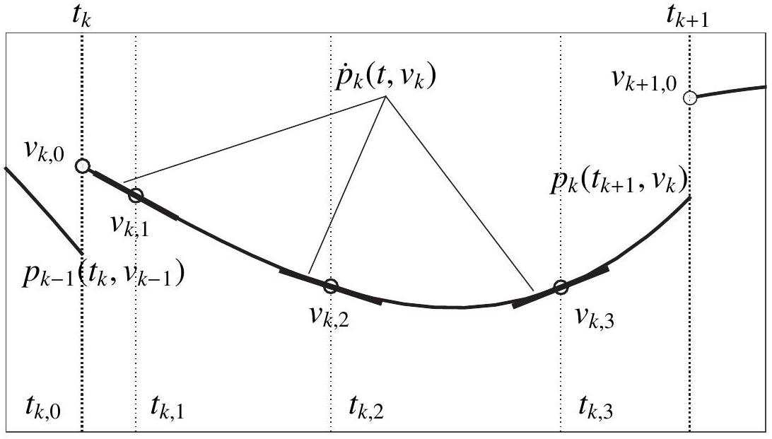
Figure 13.5: Illustration of the variables and constraints of NLP (13.5) for $d=3$, and for one specific time interval $[t_k,t_{k+1}]$ before the constraints are fulfilled (early iteration). One can observe that the continuity conditions $p_k(t_{k+1},{\mathit{v}}_k)-{\mathit{v}}_{k+1,0}=0$ are not (yet) satisfied.

The direct collocation method offers two ways of increasing the numerical accuracy of the integration. We need to remember here that the integration error of a Gauss-Legendre collocation scheme is of $\mathcal{O}\left({(t_{k+1}-t_k)}^{2d}\right)$ (respectively $\mathcal{O}\left({(t_{k+1}-t_k)}^{2d-1}\right)$ for the Gauss-Radau collocation scheme). In order to gain accuracy, one can therefore increase $d$ and thereby gain two orders in the integration error. Alternatively, one can reduce the size of the time intervals $[t_k,t_{k+1}]$ by e.g. a factor $\xi$ and thereby reduce the order of the integration error by a factor ${\xi }^{2d}$ (respectively ${\xi }^{2d-1}$ for the Gauss-Radau collocation scheme). However, numerical experiments often show that the conditioning of the linear algebra underlying the NLP resulting from direct collocation tends to worsen as $d$ increases beyond relatively small orders. In practice, it often appears counterproductive to use $d>4$ for complex optimal control problems.

One ought to observe here that discretizing an OCP using direct collocation allows for a fairly straightforward construction of the exact Hessian of the NLP. Indeed, one can observe that the nonlinear contributions to the constraints involved in the NLP arising from a discretization based on direct collocation are all explicitly given by the model continuous dynamics function $\mathit{f}$, the path constraints function $\mathit{s}$, and the terminal constraints function $\mathit{b}$. These functions are, in most OCPs, readily provided in their symbolic forms. It follows that assembling the Lagrange function and computing its first and second-order derivatives is fairly straightforward using any efficient symbolic computation tool such as e.g. AMPL or casADi.

Example 13.3

Let us tackle the OCP (13.1) of Example 13.1 via direct collocation. The direct collocation is implemented using a Gauss-Legendre direct collocation scheme with $d=3$. Here again, the ordering of the equality constraints and variables is important in order to get structured sparsity patterns.

In this example, the variables are ordered in time as:

$${\mathit{v}}_{0,0},\dots ,{\mathit{v}}_{0,3},{\mathit{q}}_0,\dots ,{\mathit{v}}_{N-1,0},\dots ,{\mathit{v}}_{N-1,3},{\mathit{q}}_{N-1}$$

where ${\mathit{v}}_{k,i}\in {\mathbb{R}}^2$, and the constraints are also ordered in time. The resulting solution is illustrated in Figure 13.6, together with the sparsity patterns of the Jacobian of the equality constraint function, and the one of the Hessian of the Lagrange function.

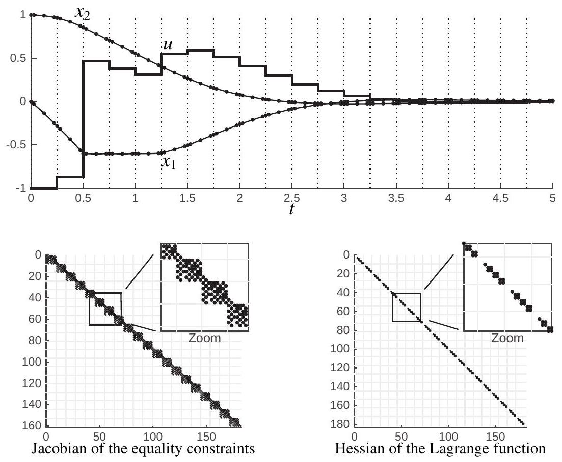
Figure 13.6: Solution to OCP $(13.1)$ using a Gauss-Legendre direct collocation discretization scheme with $d=3$, and $N=20$. The upper graph reports the states and input trajectories. The collocated states ${\mathit{v}}_{k,i}$ are reported as the dots. The lower graphs report the sparsity pattern of the Jacobian of the equality constraints in the resulting NLP and the sparsity pattern of the Hessian of the Lagrange function. Observe that the Hessian is block diagonal, while the Jacobian has a block-diagonal pattern with some elements off the blocks corresponding to the continuity conditions. The Jacobian of the inequality constraints is diagonal in this example, and block-diagonal in general.

The large NLP resulting from direct collocation need to be solved by structure exploiting solvers, and due to the fact that the problem functions are typically relatively cheap to evaluate compared to the cost of the linear algebra, nonlinear interior point methods are often the most efficient approach here. A widespread combination is to use collocation with IPOPT using the AMPL interface, or the casADi tool. It is interesting to note that, like in direct multiple shooting, the multipliers associated to the continuity conditions are again an approximation of the adjoint variables.

An interesting variant of orthogonal collocation methods that is often called the pseudo-spectral optimal control method uses only one collocation interval but on this interval it uses an extremely high order polynomial. State constraints are then typically enforced at all collocation points. Unfortunately, the constraints Jacobian and Lagrange Hessian matrices arising from the pseudospectral method are typically fairly dense and therefore more expensive to factorize than the ones arising in direct collocation.

Alternative input parametrization

We have discussed to far the use of a piecewise-constant input parametrization in the context of direct methods. We ought to stress here that, while this choice is simple and very popular, it is also arbitrary. In fact, what qualifies direct methods is their use of a restriction of the continuous (and therefore $\mathrm{\infty }$-dimensional) input profile $\mathit{\alpha }(t)$ to a space of finite dimension, which can then be described via a finite set of numbers and therefore treated in the computer. In principle, any description of the continuous input $\mathit{\alpha }(t)$ as a finite-dimensional object is possible, though some descriptions are less favorable than others. Indeed, it can e.g. be counterproductive to adopt an input discritization that destroys or degrades the sparsity patterns arising in the linear algebra of the various direct methods presented above. For this reason, it is typically preferable to adopt input discretizations that are "local" in time. Indeed, the sparsity patterns specific to the structure arising both in multiple-shooting and direct collocation hinge on the division of the overall time interval $[t_0,t_N]$ into the subintervals $[t_k,t_{k+1}]$, and the fact that the variables specific to one interval $k$, e.g. ${\mathit{v}}_k,{\mathit{q}}_k$ in the direct collocation method have an impact only on the neighboring intervals ( $k-1$ and $k+1$ ) via the continuity conditions. It would then be unwise to destroy this feature by using a discretization of the continuous input $\mathit{\alpha }(t)$ where the input parameters $\mathit{q}$ influence the input profile globally (i.e. at e.g. all time instants) such that an input parameter ${\mathit{q}}_k$ would influence all intervals. This observation rules out the use of "global" input parametrizations such as e.g. parametrizing the inputs via a finite Fourier series or a polynomial basis over the whole interval $[t_0,t_N]$.

In the context of direct collocation, a fairly natural refinement of the continuous input parametrization consists in providing as many DoF as the discretization of the optimal control problem allows. More specifically, one can readily observe that the standard piecewise input parametrization is enforced by construction of the collocation equations $(13.4)$, where a single input value ${\mathit{q}}_k$ is used on each collocation interval $[t_k,t_{k+1}]$. More DoF in the discretized input can, however, be readily added by allowing a different input ${\mathit{q}}_{k,i}$ at every collocation time point $t_{k,i}$, for $i=1,\dots ,d$. The collocation equations for each interval $k=0,\dots ,N-1$ then read as:

$${\mathit{c}}_k({\mathit{v}}_k,{\mathit{\beta }}_k,{\mathit{q}}_k)=\left[\begin{array}{c}{\mathit{v}}_{k,0}-{\mathit{\beta }}_k\\ {\dot{\mathit{p}}}_k(t_{k,i},{\mathit{v}}_k)-\mathit{f}({\mathit{v}}_{k,i},t_{k,i},{\mathit{q}}_{k,i})\\ ⋮\\ {\dot{\mathit{p}}}_k(t_{k,d},{\mathit{v}}_k)-\mathit{f}({\mathit{v}}_{k,d},t_{k,d},{\mathit{q}}_{k,d})\end{array}\right]=0.$$

and the NLP receives the decision variables

$$w=\{{\mathit{v}}_{0,0},{\mathit{v}}_{0,1},{\mathit{q}}_{0,1},\dots {\mathit{v}}_{0,d},{\mathit{q}}_{0,d},{\mathit{v}}_{1,0},{\mathit{v}}_{1,1},{\mathit{q}}_{1,1},\dots ,{\mathit{v}}_{1,d},{\mathit{q}}_{1,d},\dots \}.$$

It is important to observe here that the input is parametrized as ${\mathit{q}}_{k,i}$ with $k=0,\dots ,N-1$ and $i=1,\dots ,d$, i.e. no degree of freedom ${\mathit{q}}_{k,0}$ ought to be attributed to the discrete input on the first collocation times $t_{k,0}$, as only the continuity of the state trajectory is enforced on that collocation time.

7.4 A Classification of Direct Optimal Control Methods

It is an interesting exercise to try to classify Newton type optimal control algorithms. Let us have a look at how nonlinear optimal control algorithms perform their major algorithmic components, each of which comes in several variants:

• Treatment of Inequalities: Nonlinear integer program (IP) vs. SQP.
• Nonlinear Iterations: Simultaneous vs. Sequential.
• Derivative Computations: Full vs. Reduced.
• Linear Algebra: Banded vs. Condensing.

In the last two of these categories, we observe that the first variants each exploit the specific structures of the simultaneous approach, while the second variant reduces the variable space to the one of the sequential approach. Note that reduced derivatives imply condensed linear algebra, so the combination [Reduced,Banded] is excluded. In the first category, we might sometimes distinguish two variants of SQP methods, depending on how they solve their underlying QP problems, via active set QP solvers (SQP-AS) or via interior point methods (SQP-IP).

Based on these four categories, each with two alternatives, and one combination excluded, we obtain 12 possible combinations. In these categories, the classical single shooting method could be classified as [SQP, Sequential, Reduced] or as [SQP, Sequential, Full, Condensing] because some variants compute directly the reduced derivatives $R^u$, while others compute first the stagewise derivative matrices $M_i$ and $N_i$ and condense then. Tenny’s feasibility perturbed SQP method could be classified as [SQP, Sequential, Full, Banded], and Bock’s multiple shooting as well as the classical reduced SQP collocation methods as [SQP, Simultaneous, Full, Condensing]. The band structure exploiting SQP variants from Steinbach and Franke are classified as [SQP-IP, Simultaneous, Full, Banded], while the widely used interior point direct collocation method in conjunction with IPOPT by Biegler and W¨achter as [IP, Simultaneous, Full, Banded]. The reduced Gauss-Newton method of Schl¨oder would here be classified as [SQP, Simultaneous, Reduced]