Fluid Kinematics

• Statics: $\sum F=0$
• Dynamics: $\sum F=ma$
• Kinematics:$$\begin{array}{c}v=u+at\\ S=ut+\frac{1}{2}a{t}^2\\ v^2-u^2=2aS\end{array}$$

1. Kinematics: The study of motion
2. Fluid Kinematics: The study of how fluids flow and how to describe fluid motion.
3. Fluid particle: When we speak of a fluid particle or fluid element we are not referring to a single molecule. Rather, we mean some volume of fluid that is small by macroscopic standards, but nonetheless contains many molecules. The properties of such a fluid particle are insensitive to the behavior of any one molecule.

Lagrangian and Eulerian Description

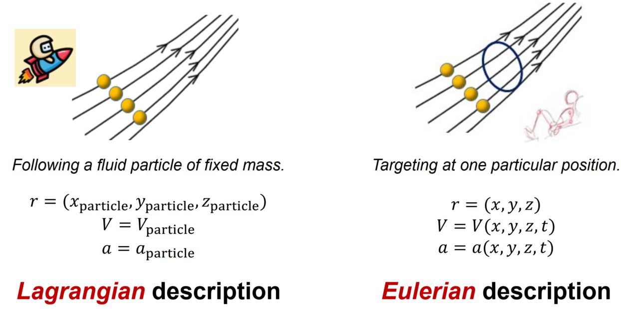
• The Lagrangian Description is one in which individual fluid particles are tracked
• The Eulerian Description is one in which a control volume is defined, within which fluid flow properties of interest are expressed as field

Two distinct ways to describe motion

Lagrangian description:

• With a small number of objects, such as billiard balls on a pool table, individual objects can be tracked
• In the Lagrangian description, one must keep track of the position and velocity of individual particles.

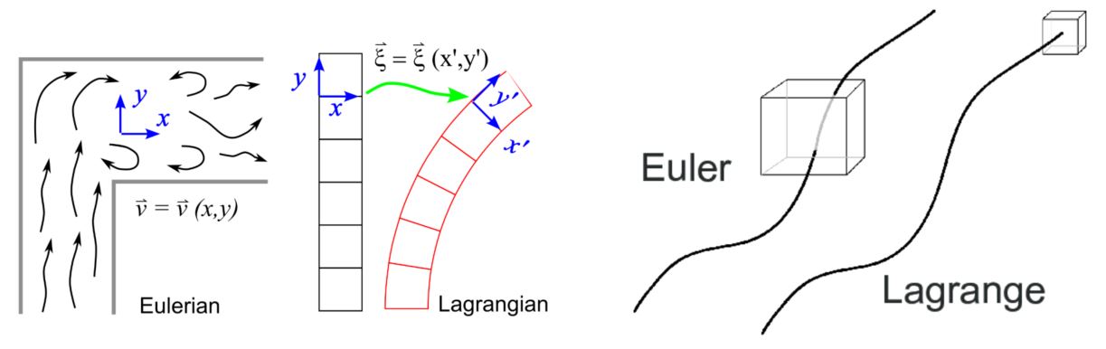
Eulerian description: Use the concept of field variables, e.g.,

$$\begin{array}{rlrl}& \text{Pressure field}:& & P=P(x,y,z,t)\\ & \text{Velocity field}:& & \overrightarrow{V}=\overrightarrow{V}(x,y,z,t)\\ & \text{Acceleration field}:& & \overrightarrow{a}=\overrightarrow{a}(x,y,z,t)\end{array}$$

• The pressure field is a scalar field variable, while the velocity and acceleration are vector variables.
• The field variable at a particular location at a particular time is the value of the variable for whichever fluid particle happens to occupy that location at that time.

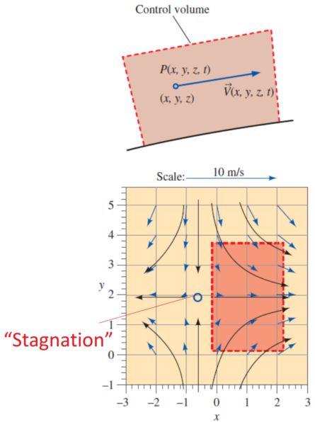
For example, the pressure field is a scalar field variable. We define the velocity field as a vector field variable. In the Eulerian description of fluid flow, a finite volume called a flow domain or control volume is defined, through which fluid flows in and out.

Instead of tracking individual fluid particles, we define field variables, functions of space and time, within the control volume.

Experimental measurements are generally more suited to the Eulerian description. Collectively, field variables define the flow field.

For example, a steady two-dimensional velocity field,

$$\overrightarrow{V}=(u,v)=(0.5+0.8x)\overrightarrow{ı}+(1.5-0.8y)\overrightarrow{ȷ}.$$

A stagnation point of zero velocity at (-0.625, 1.875).

Acceleration field

The acceleration of a fluid particle passing a position $(x,y,z)$ is

$$\overrightarrow{a}=\frac{\mathrm{d}\overrightarrow{V}}{\mathrm{d}t}$$

The velocity variable is a function of space and time: $\overrightarrow{V}=f(x,y,z,t)$

Thus, the full differential expression of the acceleration is,

$$\overrightarrow{a}=\frac{\mathrm{d}\overrightarrow{V}}{\mathrm{d}t}=\frac{\partial \overrightarrow{V}}{\partial t}\frac{\mathrm{d}t}{\mathrm{d}t}+\frac{\partial \overrightarrow{V}}{\partial x}\frac{\mathrm{d}x}{\mathrm{d}t}+\frac{\partial \overrightarrow{V}}{\partial y}\frac{\mathrm{d}y}{\mathrm{d}t}+\frac{\partial \overrightarrow{V}}{\partial z}\frac{\mathrm{d}z}{\mathrm{d}t}$$

Put $u,v,w$ are the velocity components in the $x,y,z$ directions as:

$$u=\frac{\mathrm{d}x}{\mathrm{d}t},v=\frac{\mathrm{d}y}{\mathrm{d}t},w=\frac{\mathrm{d}z}{\mathrm{d}t}$$

and

$$\begin{array}{rl}\overrightarrow{a}& =\frac{\mathrm{d}\overrightarrow{V}}{\mathrm{d}t}=\frac{\partial \overrightarrow{V}}{\partial t}+u\frac{\partial \overrightarrow{V}}{\partial x}+v\frac{\partial \overrightarrow{V}}{\partial y}+w\frac{\partial \overrightarrow{V}}{\partial z}\\ & =\frac{\partial \overrightarrow{V}}{\partial t}+(\overrightarrow{V}\cdot \overrightarrow{\mathrm{\nabla }})\overrightarrow{V}\end{array}$$

where

$$\overrightarrow{\mathrm{\nabla }}=(\frac{\partial }{\partial x},\frac{\partial }{\partial y},\frac{\partial }{\partial z})=\overrightarrow{ı}\frac{\partial }{\partial x}+\overrightarrow{ȷ}\frac{\partial }{\partial y}+\overrightarrow{k}\frac{\partial }{\partial z}$$

In Cartesian coordinates:

$$\begin{array}{rl}{a}_x& =\frac{\partial u}{\partial t}+u\frac{\partial u}{\partial x}+v\frac{\partial u}{\partial y}+w\frac{\partial u}{\partial z}\\ a_y& =\frac{\partial v}{\partial t}+u\frac{\partial v}{\partial x}+v\frac{\partial v}{\partial y}+w\frac{\partial v}{\partial z}\\ a_z& =\frac{\partial w}{\partial t}+u\frac{\partial w}{\partial x}+v\frac{\partial w}{\partial y}+w\frac{\partial w}{\partial z}\end{array}$$

It can be divided as [core]

• local acceleration $(\partial \ast /\partial t)$: it's the change in velocity w.r.t. time in a fluid flow

  • Local acceleration results when the flow is unsteady, because it is associated with temporal gradients of velocity in the flow field.

• advective / convective acceleration (others): it's the velocity at a point multiplied with the velocity gradient at that point within the fluid flow

  • The acceleration variable can be nonzero even for steady flows due to the advective term.
  • Convective acceleration results when the flow is non-uniform, that is, if the velocity changes along a streamline.

Example1 [core]

A girl is washing her car using a nozzle, which is $9.91\mathrm{cm}$ long, with an inlet diameter of $1.07\mathrm{cm}$ and an outlet diameter of $0.460\mathrm{cm}$. The volume flow rate $\dot{V}$ through the garden hose (and through the nozzle) is $0.0530\mathrm{L}/\mathrm{s}$, and the flow is steady.

Estimate the magnitude of the acceleration of the water jet at the outlet of the nozzle.

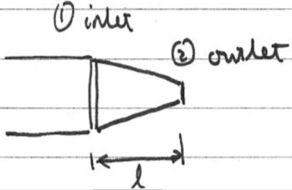
Soultion: Given

$$\begin{array}{rl}\dot{V}& =0.053\mathrm{L}/\mathrm{s}=5.3\times {10}^{-5}{\mathrm{m}}^3/\mathrm{s}\\ d_1& =0.0107\mathrm{m}\\ d_2& =0.0046\mathrm{m}\\ l& =0.0991\mathrm{m}\end{array}$$

Then

$$A_1=\frac{\pi d_1^2}{4}=8.992\times {10}^{-5}{\mathrm{m}}^2;A_2=1.662{\mathrm{m}}^2$$

Since

$$\dot{V}=A_1{V}_1=A_2{V}_2$$

Thus

$$\begin{array}{rl}{V}_1& =\frac{\dot{V}}{A_1}=0.5894\mathrm{m}/\mathrm{s}\\ V_2& =3.189\mathrm{m}/\mathrm{s}\end{array}$$

Since

$$a_x=\text{⧸}\frac{\partial u}{\partial t}+u\frac{\partial u}{\partial x}+\mathrm{v̸}\frac{\partial u}{\partial y}+\mathrm{w̸}\frac{\partial u}{\partial z}$$

By approximation

$$\begin{array}{rl}{a}_x& =u_{\mathrm{avg}}\left(\frac{u_2-u_1}{l}\right)=\left(\frac{u_2+u_1}{2}\right)\left(\frac{u_2-u_1}{l}\right)\\ & =\frac{u_2^2-u_1^2}{2l}=\frac{{3.189}^2-{0.5894}^2}{2(0.0991)}=49.6\mathrm{m}/{\mathrm{s}}^2\end{array}$$

Material derivative

Material derivation is also known as substantial derivative. It is denoted as $\mathrm{D}/\mathrm{D}t$, and illustrates the total derivative operator $\mathrm{d}/\mathrm{d}t$ such that

$$\frac{\mathrm{D}}{\mathrm{D}t}=\frac{\mathrm{d}}{\mathrm{d}t}=\frac{\partial }{\partial t}+(\overrightarrow{V}\cdot \overrightarrow{\mathrm{\nabla }})$$

Thus the material acceleration is:

$$\overrightarrow{a}(x,y,z,t)=\frac{\mathrm{D}\overrightarrow{V}}{\mathrm{D}t}=\frac{\mathrm{d}\overrightarrow{V}}{\mathrm{d}t}=\frac{\partial \overrightarrow{V}}{\partial t}+(\overrightarrow{V}\cdot \overrightarrow{\mathrm{\nabla }})\overrightarrow{V}$$

and the material derivative of pressure is:

$$\frac{\mathrm{D}P}{\mathrm{D}t}=\frac{\mathrm{d}P}{\mathrm{d}t}=\frac{\partial P}{\partial t}+(\overrightarrow{V}\cdot \overrightarrow{\mathrm{\nabla }})P$$

The Material Derivative, in engineering, is a derivative taken along a path moving with velocity field. It measures the rate of change experienced by a physical quantity, like temperature or velocity, associated with the motion of the material within a flow field.

The material derivative describes the time rate of change of some physical quantity (e.g heat) of a material element that is subjected to a space-and-time-dependent macroscopic velocity field. The material derivative can serve as a link between Eulerian and Lagrangian descriptions of continuum deformation.

e.g. The material acceleration of a steady velocity field,

$$\overrightarrow{V}=(u,v)=(0.5+0.8x)\overrightarrow{ı}+(1.5-0.8y)\overrightarrow{ȷ}$$$$\begin{array}{rlrlrl}{a}_x& =\frac{\partial u}{\partial t}+u\frac{\partial u}{\partial x}& & +v\frac{\partial u}{\partial y}& & +w\frac{\partial u}{\partial z}\\ a_x& =0+\overbrace{(0.5+0.8x)(0.8)}& & +\overbrace{(1.5-0.8y)(0)}& & +0=(0.4+0.64x)\mathrm{m}/{\mathrm{s}}^2\end{array}$$$$\begin{array}{rlrlrl}& a_y=\frac{\partial v}{\partial t}+u\frac{\partial v}{\partial x}& & +v\frac{\partial v}{\partial y}& & +w\frac{\partial v}{\partial z}\\ & a_y=0+\overbrace{(0.5+0.8x)(0)}& & +\overbrace{(1.5-0.8y)(-0.8)}& & +0=(-1.2+0.64y)\mathrm{m}/{\mathrm{s}}^2\end{array}$$

Say at point $(2,3)$. The acceleration: $a_x=1.68\mathrm{m}/{\mathrm{s}}^2$ and $a_y=1.720\mathrm{m}/{\mathrm{s}}^2$.

The steady flow field:

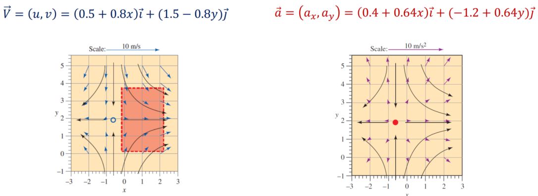
Example2

A steady, incompressible, two-dimensional velocity field is,

$$\overrightarrow{V}=(u,v)=(1.9+2.1x+0.66y)\overrightarrow{ı}+(0.75-2.2x-2.1y)\overrightarrow{ȷ}$$

Calculate the acceleration field ($a_x$ and $a_y$), and calculate the acceleration at the point $(x,y)=(-1,3)$ .

Solution:

$$\begin{array}{rl}u& =1.9+2.1x+0.66y\\ v& =0.75-2.2x-2.1y\end{array}$$

Then

$$\begin{array}{rlrl}\frac{\partial u}{\partial x}& =2.1,& \frac{\partial u}{\partial y}& =0.66\\ \frac{\partial v}{\partial x}& =-2.2,& \frac{\partial v}{\partial y}& =-2.1\end{array}$$

Thus

$$\begin{array}{rl}{a}_x=& \frac{\partial u}{\partial t}+u\frac{\partial u}{\partial x}+v\frac{\partial u}{\partial y}\\ =& 0+(1.9+2.1x+0.66y)(2.1)\\ & +(0.75-2.2x-2.1y)(0.66)\\ =& 4.49+2.96x\end{array}$$$$\begin{array}{rl}{a}_y=& \frac{\partial v}{\partial t}+u\frac{\partial v}{\partial x}+v\frac{\partial v}{\partial y}\\ =& 0+(1.9+2.1x+0.66y)(-2.2)\\ & +(0.75-2.2x-2.1y)(-2.1)\\ =& -5.76+2.96y\end{array}$$

Thus, at $(-1,3)$:

$$\begin{array}{rl}{a}_x& =4.49+2.96(-1)=1.5\\ a_y& =-5.76+2.96(3)=3.1\end{array}$$

Flow Patterns and Flow Visualization

Definition: Flow Visualization

The visual examination of flow field features

Quantitative study of fluid dynamics requires advanced mathematics and in fact, much can be learned from flow visualization.

Flow visualization is useful not only in physical experiments but in numerical solutions as well computational fluid dynamics (CFD).

In fact, the very first thing an engineer using CFD does after obtaining a numerical solution is to simulate some form of flow visualization.

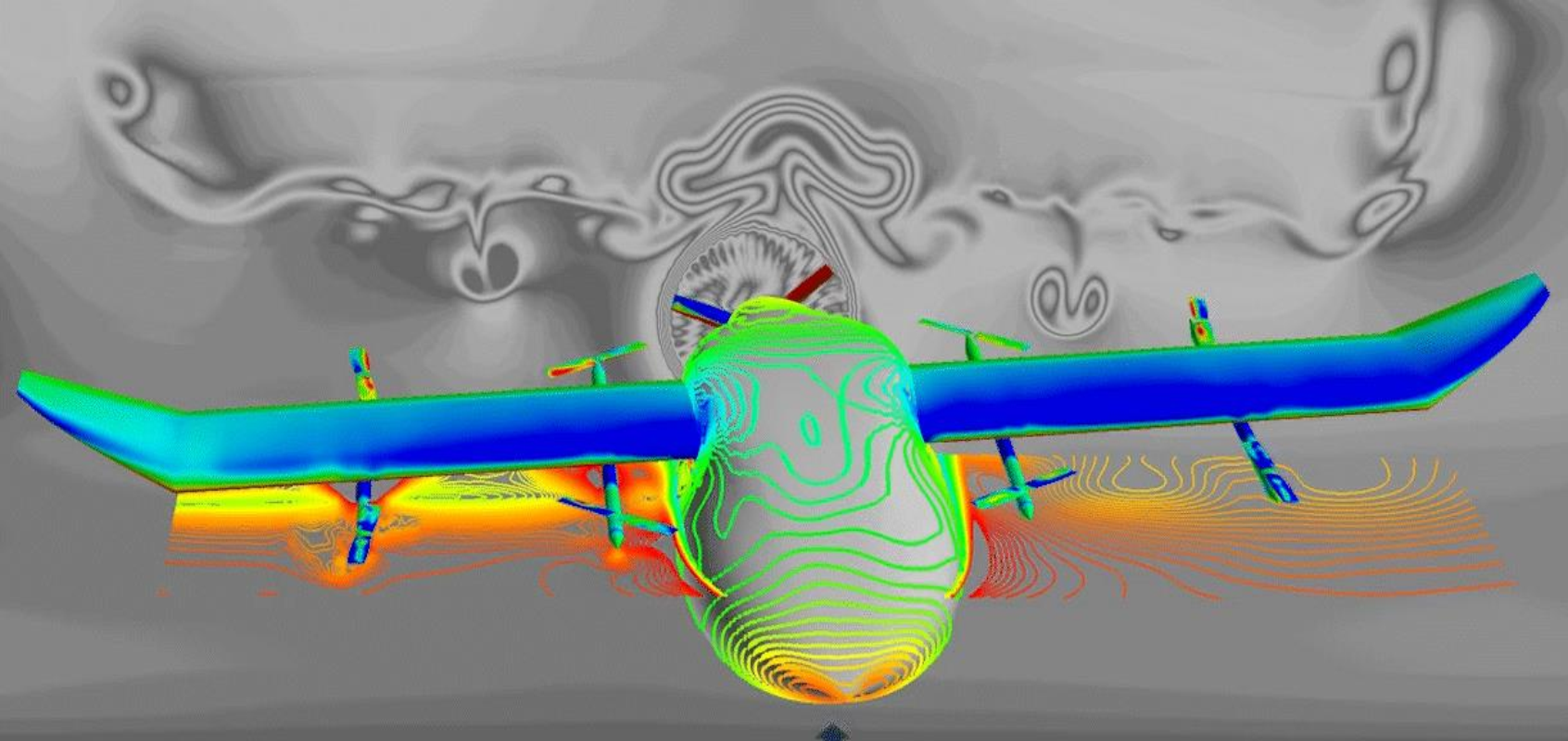
The figure above is that NASA Simulates a Smooth Ride to Stabilize Air Taxis.

Streamlines and streamtubes

Definition: streamline

Streamline: A curve that

• all the particles at any point have the same speed at any particular instant; and
• has tangent at all points to be in the same direction of the instantaneous local velocity vector.

• Streamlines are useful as indicators of the instantaneous direction of fluid motion throughout the flow field.
• Streamlines can only be observed experimentally in steady flow fields, but not in unsteady flow fields.
• Streamlines are a family of curves whose tangent vectors constitute the velocity vector field of the flow. These show the direction in which a massless fluid element will travel at any point in time

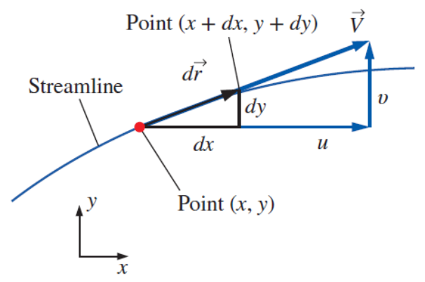
Consider an infinitesimal arc length, $\mathrm{d}\overrightarrow{r}$ approaches to the direction of $\overrightarrow{V}$,

$$\frac{\mathrm{d}r}{V}=\frac{\mathrm{d}x}{u}=\frac{\mathrm{d}y}{v}$$

Thus the equation for a streamline:

$$\frac{\mathrm{d}x}{u}=\frac{\mathrm{d}y}{v}=\frac{\mathrm{d}z}{w}$$

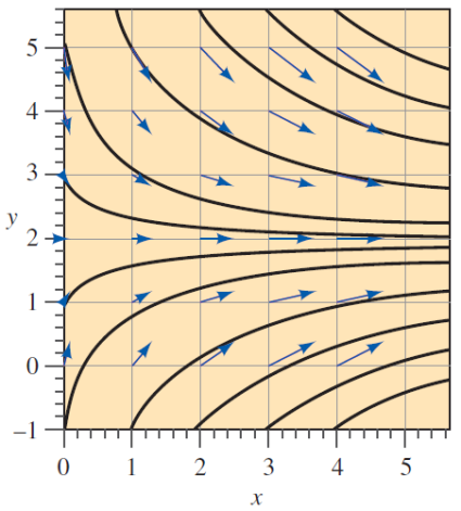
Example3

A steady, incompressible, two-dimensional velocity field,

$$\overrightarrow{V}=(u,v)=(0.5+0.8x)\overrightarrow{ı}+(1.5-0.8y)\overrightarrow{ȷ}$$

Obtain the equation of the streamlines and plot the streamlines from $x>0$.

Solution: For the streamline equation:

$$\begin{array}{rl}\frac{\mathrm{d}x}{u}& =\frac{\mathrm{d}y}{v}\\ ⟹\frac{\mathrm{d}x}{0.5+0.8x}& =\frac{\mathrm{d}y}{1.5-0.8y}\\ ⟹\int \frac{\mathrm{d}x}{0.5+0.8x}& =\int \frac{\mathrm{d}y}{1.5-0.8y}\\ ⟹\frac{1}{0.8}\int \frac{\mathrm{d}(0.5+0.8x)}{0.5+0.8x}& =\frac{1}{-0.8}\int \frac{\mathrm{d}(1.5-0.8y)}{1.5-0.8y}\\ ⟹\frac{1}{0.8}\ln (0.5+0.8x)& =\frac{1}{-0.8}\ln (1.5-0.8y)+C\end{array}$$$$\begin{array}{rl}& \frac{\ln (0.5+0.8x)+\ln (1.5-0.8y)}{0.8}=C\\ ⟹& \ln [(0.5+0.8x)(1.5-0.8y)]=C_1\\ ⟹& (0.5+0.8x)(1.5-0.8y)=C_2\\ ⟹& 1.5-0.8y=\frac{C_2}{0.5+0.8x}\\ ⟹& y=\frac{C_3}{0.8(0.5+0.8x)}+1.875\end{array}$$

$C_3$ is a constant that can be set to various values.

---

Above is the edge of the mid-term test