3 Linear time-Optimal Control

3.1 Existence of Time-Optimal Control

Consider the linear system of ODE:

$$\{\begin{array}{l}\dot{\mathit{x}}(t)=M\mathit{x}(t)+N\mathit{\alpha }(t)\\ \mathit{x}(0)=x^0,\end{array}$$

for given matrices $M\in {\mathbb{M}}^{n\times n}$ and $N\in {\mathbb{M}}^{n\times m}$. We'll again take $A$ to be the cube $[-1,1{]}^m\subset {\mathbb{R}}^m$.

Define next

$$P[\mathit{\alpha }(\cdot )]:=-{\int }_0^{\tau }1\mathrm{d}s=-\tau ,$$

where $\tau =\tau (\mathit{\alpha }(\cdot ))$ denotes the first time the solution of our system hits the origin $0$. (If the trajectory never hits $0$, we set $\tau =\mathrm{\infty }$.)

Optimal Control Problem

We are given the starting point $x^0\in {\mathbb{R}}^n$, and want to find an optimal control ${\mathit{\alpha }}^{\ast }(\cdot )$ s.t.

$$P[{\mathit{\alpha }}^{\ast }(\cdot )]=\underset{\mathit{\alpha }(\cdot )\in \mathcal{A}}{max}P[\mathit{\alpha }(\cdot )].$$

Then ${\tau }^{\ast }=-\mathcal{P}[{\mathit{\alpha }}^{\ast }(\cdot )]$ is the minimum time to steer to the origin.

Theorem 3.1: Existence of Time-Optimal Control

Let $x^0\in {\mathbb{R}}^n$. Then there exists an optimal bang-bang control ${\mathit{\alpha }}^{\ast }(\cdot )$.

Proof: Let ${\tau }^{\ast }:=inf\{t|x^0\in \mathcal{C}(t)\}$. We want to show that $x^0\in \mathcal{C}({\tau }^{\ast })$; that is, there exists an optimal control ${\mathit{\alpha }}^{\ast }(\cdot )$ steering $x^0$ to $0$ at time ${\tau }^{\ast }$.

Coose $t_1\ge t_2\ge t_3\ge \cdots$ s.t. $x^0\in \mathcal{C}(t_n)$ and $t_n\to {\tau }^{\ast }$. Since $x^0\in \mathcal{C}(t_n)$, there exists a control ${\mathit{\alpha }}_n(\cdot )\in \mathcal{A}$ s.t.

$$x^0=-{\int }_0^{t_n}{\mathit{X}}^{-1}(s)N{\mathit{\alpha }}_n(s)\mathrm{d}s.$$

If necessary, redefine ${\mathit{\alpha }}_n(s)$ to be $0$ for $s\ge t_n$. By Alaoglu’s Theorem, there exists a subsequence $n_k\to \mathrm{\infty }$ and a control ${\mathit{\alpha }}^{\ast }(\cdot )$ s.t.

$${\mathit{\alpha }}_n\stackrel{\ast }{\rightharpoonup }{\mathit{\alpha }}^{\ast }.$$

We assert that ${\mathit{\alpha }}^{\ast }(\cdot )$ is an optimal control. It is easy to check that ${\mathit{\alpha }}^{\ast }(s)=0,s\ge {\tau }^{\ast }$. Also

$$x^0=-{\int }_0^{t_{n_k}}{\mathit{X}}^{-1}(s)N{\mathit{\alpha }}_{n_k}(s)\mathrm{d}s=-{\int }_0^{t_1}{\mathit{X}}^{-1}(s)N{\mathit{\alpha }}_{n_k}(s)\mathrm{d}s,$$

Since ${\mathit{\alpha }}_{n_k}=0$ for $s\ge t_{n_k}$. let $n_k\to \mathrm{\infty }$:

$$x^0=-{\int }_0^{t_1}{\mathit{X}}^{-1}(s)N{\mathit{\alpha }}^{\ast }(s)\mathrm{d}s=-{\int }_0^{{\tau }^{\ast }}{\mathit{X}}^{-1}(s)N{\mathit{\alpha }}^{\ast }(s)\mathrm{d}s$$

because ${\mathit{\alpha }}^{\ast }(s)=0$ for $s\ge {\tau }^{\ast }$. Hence $x^0\in \mathcal{C}({\tau }^{\ast })$, and therefore ${\mathit{\alpha }}^{\ast }(\cdot )$ is optimal.

According to Theorem 2.10 there in fact exists an optimal bang-bang control.

$◻$

3.2 The Maximum Principle for Linear Time-Optimal Control

The really interesting practical issue now is understanding how to compute an optimal control ${\mathit{\alpha }}^{\ast }(\cdot )$.

Definition

Define $K(t,x^0)$ to be the reachable set for time $t$. That is:

$$K(t,x^0)=\{x^1|\text{there exists }\mathit{\alpha }(\cdot )\in \mathcal{A}\text{ which steers from }{x}^0\text{ to }{x}^1\text{ at time }t\}.$$

Since $\mathit{x}(\cdot )$ solves ODE, we have $x^1\in K(t,x^0)$ iff

$$x^1=\mathit{X}(t)x^0+\mathit{X}(t){\int }_0^t{\mathit{X}}^{-1}(s)N\mathit{\alpha }(s)\mathrm{d}s=\mathit{x}(t)$$

for some control $\mathit{\alpha }(\cdot )\in \mathcal{A}$.

Theorem 3.2: Geometry of the set $K$

The set $K(t,x^0)$ is convex and closed.

Proof:

1. (convexity) Let $x^1,x^2\in K(t,x^0)$. Then $\mathrm{\exists }{\mathit{\alpha }}_1,{\mathit{\alpha }}_2\in \mathcal{A}$ s.t.

$$\begin{array}{rl}{x}^1& =\mathit{X}(t)x^0+\mathit{X}(t){\int }_0^t{\mathit{X}}^{-1}(s)N{\mathit{\alpha }}_1(s)\mathrm{d}s\\ x^2& =\mathit{X}(t)x^0+\mathit{X}(t){\int }_0^t{\mathit{X}}^{-1}(s)N{\mathit{\alpha }}_2(s)\mathrm{d}s,\end{array}$$

Let $0\le \lambda \le 1$. Then

$$\lambda x^1+(1-\lambda )x^2=\mathit{X}(t)x^0+\mathit{X}(t){\int }_0^t{\mathit{X}}^{-1}(s)N\underset{\in \mathcal{A}}{\underbrace{(\lambda {\mathit{\alpha }}_1(s)+(1-\lambda ){\mathit{\alpha }}_2(s))}}\mathrm{d}s,$$

and hence $\lambda x^1+(1-\lambda )x^2\in K(t,x^0)$.

2. (Closedness) Assume $x^k\in K(t,x^0)$ for $(k=1,2,\cdots )$ and $x^k\to y$. We must show $y\in K(t,x^0)$. As $x^k\in K(t,x^0)$. As $x^k\in K(t,x^0),\mathrm{\exists }{\mathit{\alpha }}_k\in \mathcal{A}$ s.t.

$$x^k=\mathit{X}(t)x^0+\mathit{X}(t){\int }_0^t{\mathit{X}}^{-1}(s)N{\mathit{\alpha }}_k(s)\mathrm{d}s.$$

According to Alaoglu’s Theorem, there exist a subsequence $k_j\to \mathrm{\infty }$ and $\mathit{\alpha }\in \mathcal{A}$ s.t. ${\mathit{\alpha }}_k\stackrel{\ast }{\rightharpoonup }\mathit{\alpha }$. Let $k=k_j\to \mathrm{\infty }$ in the expression above, to find

$$y=\mathit{X}(t)x^0+\mathit{X}(t){\int }_0^t{\mathit{X}}^{-1}(s)N\mathit{\alpha }(s)\mathrm{d}s.$$

Thus $y\in K(t,x^0)$, an hence $K(t,x^0)$ is closed.

$◻$

Notation: boundary

If $S$ is a set, we write $\partial S$ to denote the boundary of $S$.

Recall that ${\tau }^{\ast }$ denotes the minimum time it takes to steer to 0, using the optimal control ${\mathit{\alpha }}^{\ast }$. Note that then $0\in \partial K({\tau }^{\ast },x^0)$.

Theorem 3.3: Portryagin Maximum Prnciple for Linear Time-Optimal Control

there exists a nonzero vector $\mathit{h}$ s.t.

$$\begin{array}{}\text{(M)}& {\mathit{h}}^{\mathrm{\top }}{\mathit{X}}^{-1}(t)N{\mathit{\alpha }}^{\ast }(t)=\underset{a\in A}{max}\{{\mathit{h}}^{\mathrm{\top }}{\mathit{X}}^{-1}(t)Na\}.\end{array}$$

for each time $0\le t\le {\tau }^{\ast }$.

Interpretation: The significance of this assertion is that if we know $\mathit{h}$ then the maximization principle (M) provides us with a formula for computing ${\mathit{\alpha }}^{\ast }(\cdot )$, or at least extracting useful information.

We will see in the next chapter that assertion (M) is a special case of the general Pontryagin Maximum Principle.

Proof:

1. We know $0\in \partial K({\tau }^{\ast },x^0)$. Since $K({\tau }^{\ast },x^0)$ is convex, There exist a supporting plane to $K({\tau }^{\ast },x^0)$ at $0$; this means tat for some $\mathit{g}\ne 0$, we have

$$\mathit{g}\cdot x_1\le 0,\mathrm{\forall }{x}_1\in K({\tau }^{\ast },x^0).$$

2. Now $x^1\in K({\tau }^{\ast },x^0)$ iff $\mathrm{\exists }\mathit{\alpha }(\cdot )\in \mathcal{A}$ s.t.

$$x^1=\mathit{X}({\tau }^{\ast })x^0+\mathit{X}({\tau }^{\ast }){\int }_0^{{\tau }^{\ast }}{\mathit{X}}^{-1}(s)N\mathit{\alpha }(s)\mathrm{d}s.$$

Also

$$0=\mathit{X}({\tau }^{\ast })x^0+\mathit{X}({\tau }^{\ast }){\int }_0^{{\tau }^{\ast }}{\mathit{X}}^{-1}(s)N{\mathit{\alpha }}^{\ast }(s)\mathrm{d}s.$$

Since $\mathit{g}\cdot x^1\le 0$, we deduce that

$$\begin{array}{rl}& {\mathit{g}}^{\mathrm{\top }}(\mathit{X}({\tau }^{\ast })x^0+\mathit{X}({\tau }^{\ast }){\int }_0^{{\tau }^{\ast }}{\mathit{X}}^{-1}(s)N\mathit{\alpha }(s)\mathrm{d}s)\\ \le & 0=\mathit{X}({\tau }^{\ast })x^0+\mathit{X}({\tau }^{\ast }){\int }_0^{{\tau }^{\ast }}{\mathit{X}}^{-1}(s)N{\mathit{\alpha }}^{\ast }(s)\mathrm{d}s.\end{array}$$

Define ${\mathit{h}}^{\mathrm{\top }}={\mathit{g}}^{\mathrm{\top }}\mathit{X}({\tau }^{\ast })$. Then

$${\int }_0^{{\tau }^{\ast }}{\mathit{h}}^{\mathrm{\top }}{\mathit{X}}^{-1}(s)N\mathit{\alpha }(s)\mathrm{d}s\le {\int }_0^{{\tau }^{\ast }}{\mathit{h}}^{\mathrm{\top }}{\mathit{X}}^{-1}(s)N{\mathit{\alpha }}^{\ast }(s)\mathrm{d}s;$$

and therefore

$${\int }_0^{{\tau }^{\ast }}{\mathit{h}}^{\mathrm{\top }}{\mathit{X}}^{-1}(s)N({\mathit{\alpha }}^{\ast }-\mathit{\alpha }(s))\mathrm{d}s\ge 0$$

for all controls $\mathit{\alpha }(\cdot )\in \mathcal{A}$.

3. We claim now that the foregoing implies

$${\mathit{h}}^{\mathrm{\top }}{\mathit{X}}^{-1}(t)N{\mathit{\alpha }}^{\ast }(s)=\underset{a\in A}{max}\{{\mathit{h}}^{\mathrm{\top }}{\mathit{X}}^{-1}(s)Na\}$$

for almost every time $s$. For suppose not; then there would exists a subset $E\subset [0,{\tau }^{\ast }]$ of positive measure, s.t.

$${\mathit{h}}^{\mathrm{\top }}{\mathit{X}}^{-1}(t)N{\mathit{\alpha }}^{\ast }(s)<\underset{a\in A}{max}\{{\mathit{h}}^{\mathrm{\top }}{\mathit{X}}^{-1}(s)Na\}$$

for $s\in E$. Design a new control $\hat{\mathit{\alpha }}(\cdot )$ as follows:

$$\widehat{\mathbf{(}s)}=\{\begin{array}{ll}{\mathit{\alpha }}^{\ast }(s)& (s\notin E)\\ \mathit{\alpha }(s)& (s\in E)\end{array}$$

where $\mathit{\alpha }(s)$ is selected s.t.

$$\underset{a\in A}{max}\{{\mathit{h}}^{\mathrm{\top }}{\mathit{X}}^{-1}(s)Na\}={\mathit{h}}^{\mathrm{\top }}{\mathit{X}}^{-1}(t)N\mathit{\alpha }(s).$$

Then

$${\int }_E\underset{<0}{\underbrace{{\mathit{h}}^{\mathrm{\top }}{\mathit{X}}^{-1}(s)N({\mathit{\alpha }}^{\ast }-\mathit{\alpha }(s))}}\mathrm{d}s\ge 0.$$

This contradicts Step 2 above.

$◻$

For later reference, we pause here to rewrite the foregoing into different notation; this will turn out to be a special case of the general theory developed later in Chapter 4. First of all, define the Hamiltonian:

Definition: Hamiltonian

$$H(x,p,a):=(Mx+Na)\cdot p(x,p\in {\mathbb{R}}^n,a\in A).$$

Theorem 3.4: Another way to write Pontryagin Maximum Principle for Linear Time-Optimal Control

Let ${\mathit{\alpha }}^{\ast }(\cdot )$ be a time optimal control and ${\mathit{x}}^{\ast }(\cdot )$ the corresponding response.

Then there exists a function ${\mathit{p}}^{\ast }(\cdot ):[0,{\tau }^{\ast }]\to {\mathbb{R}}^n$, s.t.

$$\begin{array}{rlrl}{\dot{\mathit{x}}}^{\ast }(t)& ={\mathrm{\nabla }}_{p}H({\mathit{x}}^{\ast }(t),{\mathit{p}}^{\ast }(t),{\mathit{\alpha }}^{\ast }(t)),& & (ODE)\\ {\dot{\mathit{p}}}^{\ast }(t)& =-{\mathrm{\nabla }}_{x}H({\mathit{x}}^{\ast }(t),{\mathit{p}}^{\ast }(t),{\mathit{\alpha }}^{\ast }(t)),& & (ADJ)\\ H({\mathit{x}}^{\ast }(t),{\mathit{p}}^{\ast }(t),{\mathit{\alpha }}^{\ast }(t))& =\underset{a\in A}{max}H({\mathit{x}}^{\ast }(t),{\mathit{p}}^{\ast }(t),a).& & (M)\end{array}$$

We call (ADJ) the adjoint equations and (M) the maximization principle. The function ${\mathit{p}}^{\ast }(\cdot )$ is the costate.

Proof:

1. Select the vector $\mathit{h}$ as in Theorem 3.3, and consider the system

$$\{\begin{array}{l}{\dot{\mathit{p}}}^{\ast }(t)=-M^{\mathrm{\top }}{\mathit{p}}^{\ast }(t)\\ {\mathit{p}}^{\ast }(0)=\mathit{h}.\end{array}$$

The solution is ${\mathit{p}}^{\ast }(t)=e^{-t{M}^{\mathrm{\top }}}\mathit{h}$; and hence

$${\mathit{p}}^{\ast }(t{)}^{\mathrm{\top }}={\mathit{h}}^{\mathrm{\top }}{\mathit{X}}^{-1}(t),$$

Since ${\left(e^{-t{M}^{\mathrm{\top }}}\right)}^{\mathrm{\top }}=e^{-tM}={\mathit{X}}^{-1}(t)$.

2. We know from condition (M) in Theorem 3.3 that

$${\mathit{h}}^{\mathrm{\top }}{\mathit{X}}^{-1}(t)N{\mathit{\alpha }}^{\ast }(t)=\underset{a\in A}{max}\{{\mathit{h}}^{\mathrm{\top }}{\mathit{X}}^{-1}(t)Na\}.$$

Since ${\mathit{p}}^{\ast }(t{)}^{\mathrm{\top }}={\mathit{h}}^{\mathrm{\top }}{\mathit{X}}^{-1}(t)$, this means that

$${\mathit{p}}^{\ast }(t{)}^{\mathrm{\top }}(M{\mathit{x}}^{\ast }(t)+N{\mathit{\alpha }}^{\ast }(t))=\underset{a\in A}{max}\{{\mathit{p}}^{\ast }(t{)}^{\mathrm{\top }}(M{\mathit{x}}^{\ast }(t)+Na)\}.$$

3. Finally, we observe that according to the definition of the Hamiltonian $H$, the dynamical equations for ${\mathit{x}}^{\ast }(\cdot ),{\mathit{p}}^{\ast }(\cdot )$ take the form (ODE) and (ADJ), as stated in the Theorem.
   $◻$

3.3 Examples

Example 1: Rocket Railroad Car

We recall this example, introduced in §1.2. We have

$$\begin{array}{}\text{(ODE)}& \dot{\mathit{x}}(t)=\underset{M}{\underbrace{\left[\begin{array}{cc}0& 1\\ 0& 0\end{array}\right]}}\mathit{x}(t)+\underset{N}{\underbrace{\left[\begin{array}{c}0\\ 1\end{array}\right]}}\alpha (t)\end{array}$$

for

$$\mathit{x}(t)=(x^1(t),x^2(t){)}^{\mathrm{\top }},A=[-1,1].$$

According to the Pontryagin Maximum Principle, there exists $h\ne 0$ s.t.

$${\mathit{h}}^{\mathrm{\top }}{\mathit{X}}^{-1}(t)N{\mathit{\alpha }}^{\ast }(t)=\underset{|a|\le 1}{max}\{{\mathit{h}}^{\mathrm{\top }}{\mathit{X}}^{-1}(t)Na\}.$$

We will extract the interesting fact that an optimal control ${\alpha }^{\ast }$ switches at most one time.

We must compute $e^{tM}$. To do so, we observe:

$$M^0=I,M=\left[\begin{array}{cc}0& 1\\ 0& 0\end{array}\right]M^2=\left[\begin{array}{cc}0& 1\\ 0& 0\end{array}\right]\left[\begin{array}{cc}0& 1\\ 0& 0\end{array}\right]=\mathbf{0};$$

and therefore $M^k=0$ for all $k\ge 2$. Consequently,

$$e^{tM}=I+tM=\left[\begin{array}{cc}1& t\\ 0& 1\end{array}\right]$$

Then

$$\begin{array}{rl}{\mathit{X}}^{-1}(t)& =\left[\begin{array}{cc}1& -t\\ 0& 1\end{array}\right]\\ {\mathit{X}}^{-1}(t)N& =\left[\begin{array}{cc}1& -t\\ 0& 1\end{array}\right]\left[\begin{array}{c}0\\ 1\end{array}\right]=\left[\begin{array}{c}-t\\ 1\end{array}\right]\\ {\mathit{h}}^{\mathrm{\top }}{\mathit{X}}^{-1}(t)N=(h_1,h_2)\left[\begin{array}{c}-t\\ 1\end{array}\right]=-t{h}_1+h_2.\end{array}$$

The Maximum Principle asserts

$$(-t{h}_1+h_2){\alpha }^{\ast }(t)=\underset{|a|\le 1}{max}\{(-t{h}_1+h_2)a\};$$

and this implies that

$${\alpha }^{\ast }(t)=\mathrm{sgn}(-t{h}_1+h_2)$$

for the sign function

$$\mathrm{sgn}=\{\begin{array}{ll}1& x>0\\ 0& x=0\\ -1& x<0\end{array}$$

Therefore the optimal control ${\mathit{\alpha }}^{\ast }$ switches at most once($-t{h}_1+h_2$ is a function of $t$, i.e. a line); and if $h_1=0$, then ${\alpha }^{\ast }$ is constant.

Since the optimal control switches at most once, then the control we constructed by a geometric method in §1.3 must have been optimal.

$◻$

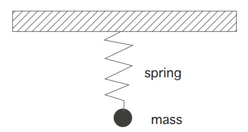
Example 2: Control of a Vibrating Spring

Consider next thesimple dynamics

$$\ddot{x}+x=\alpha ,$$

where we interpret the control as an exterior force acting on an oscillating weight (of unit mass) hanging from a spring. Our goal is to design an optimal exterior forcing ${\alpha }^{\ast }(\cdot )$ that brings the motion to a stop in minimum time.

We have $n=2,m=1$. The individual dynamical equations read:

$$\{\begin{array}{l}{\dot{x}}^1(t)=x^2(t)\\ {\dot{x}}^2(t)=-x^1(t)+\alpha (t);\end{array}$$

which in vector notation become

$$\dot{\mathit{x}}(t)=\underset{M}{\underbrace{\left[\begin{array}{cc}0& 1\\ -1& 0\end{array}\right]}}\mathit{x}(t)+\underset{N}{\underbrace{\left[\begin{array}{c}0\\ 1\end{array}\right]}}\alpha (t)$$

for $|\alpha (t)|\le 1$. That is, $A=[-1,1]$.

Using the maximum principle

We employ the Pontryagin Maximum Principle, which asserts that there exists $\mathit{h}\ne 0$ s.t.

$$\begin{array}{}\text{(M)}& {\mathit{h}}^{\mathrm{\top }}{\mathit{X}}^{-1}(t)N{\mathit{\alpha }}^{\ast }(t)=\underset{|a|\le 1}{max}\{{\mathit{h}}^{\mathrm{\top }}{\mathit{X}}^{-1}(t)Na\}.\end{array}$$

To extract useful information from (M) we must compute $\mathit{X}(\cdot )$. To do so, we observe that the matrix $M$ is skew symmetric, and thus

$$M^0=I,M=\left[\begin{array}{cc}0& 1\\ -1& 0\end{array}\right]M^2=\left[\begin{array}{cc}0& 1\\ -1& 0\end{array}\right]\left[\begin{array}{cc}-1& 0\\ 0& -1\end{array}\right]=-I;$$

Therefore

$$\begin{array}{rlrl}{M}^k& =I& & \text{if }k=0,4,8,\cdots \\ M^k& =M& & \text{if }k=1,5,9,\cdots \\ M^k& =-I& & \text{if }k=2,6,\cdots \\ M^k& =-M& & \text{if }k=3,7,\cdots \end{array}$$

and consequently

$$\begin{array}{rl}{e}^{tM}& =I+tM+\frac{t^2}{2!}{M}^2+\cdots \\ & =I+tM-\frac{t^2}{2!}I-\frac{t^3}{3!}M+\frac{t^4}{4!}I+\cdots \\ & =(1-\frac{t^2}{2!}+\frac{t^4}{4!}-\cdots )I+(t-\frac{t^3}{3!}+\frac{t^5}{5!}-\cdots )M\\ & =\cos tI+\sin tM=\left[\begin{array}{cc}\cos t& \sin t\\ -\sin t& \cos t\end{array}\right].\end{array}$$

So we have

$${\mathit{X}}^{-1}(t)=\left[\begin{array}{cc}\cos t& -\sin t\\ \sin t& \cos t\end{array}\right].$$

and

$${\mathit{X}}^{-1}(t)N=\left[\begin{array}{cc}\cos t& -\sin t\\ \sin t& \cos t\end{array}\right]\left[\begin{array}{c}0\\ 1\end{array}\right]=\left[\begin{array}{c}-\sin t\\ \cos t\end{array}\right]$$

whence

$${\mathit{h}}^{\mathrm{\top }}{\mathit{X}}^{-1}(t)N=(h_1,h_2)\left[\begin{array}{c}-\sin t\\ \cos t\end{array}\right]=-h_1\sin t+h_2\cos t.$$

According to condition (M), for each time $t$ we have

$$(-h_1\sin t+h_2\cos t){\alpha }^{\ast }(t)=\underset{|a|\le 1}{max}\{(-h_1\sin t+h_2\cos t)a\}$$

Therefore

$${\alpha }^{\ast }(t)=\mathrm{sgn}(-h_1\sin t+h_2\cos t).$$

Finding the optimal control

To simplify further, we may assume $h_1^2+h_2^2=1$ (unit vector). Recall the trig identity $\sin (x+y)=\sin x\cos y+\cos x\sin y$, and choose $\delta$ s.t. $-h_1=\cos \delta ,h_2=\sin \delta$. Then

$${\alpha }^{\ast }(t)=\mathrm{sgn}(\cos \delta \sin t+\sin \delta \cos t)=\mathrm{sgn}(\sin (t+\delta )).$$

We deduce therefore that ${\alpha }^{\ast }$ switches from $+1$ to $-1$, and vice versa, every $\pi$ units of time.

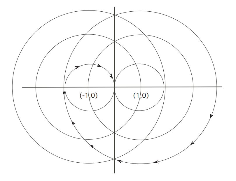
Geometric interpretation

Next, we figure out the geometric consequences.

• When $\alpha \equiv 1$, our (ODE) becomes

  $$\{\begin{array}{l}{\dot{x}}^1=x^2\\ {\dot{x}}^2=-x^1+1\end{array}$$

  In this case, we can calculate that

  $$\begin{array}{rl}\frac{\mathrm{d}}{\mathrm{d}t}[(x^1(t)-1{)}^2+(x^2(t){)}^2]& =2(x^1(t)-1){\dot{x}}^1(t)+2x^2(t){\dot{x}}^2(t)\\ & =2(x^1(t)-1)x^2(t)+2x^2(t)(-x^1(t)+1)=0.\end{array}$$

  Consequently, the motion satisfies $(x^1(t)-1{)}^2+(x^2(t){)}^2\equiv r_1^2$, for some radius $r_1$, and therefore the trajectory lies on a circle with center $(1,0)$, as illustrated.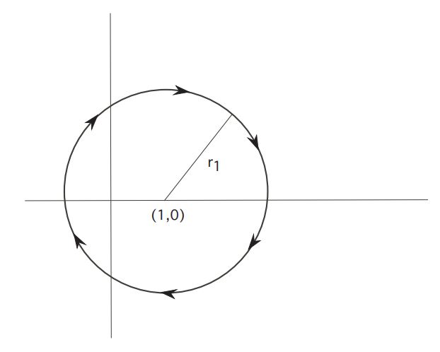

• If $\alpha \equiv -1$, our (ODE) instead becomes

  $$\{\begin{array}{l}{\dot{x}}^1=x^2\\ {\dot{x}}^2=-x^1-1\end{array}$$

  In which case

  $$\frac{\mathrm{d}}{\mathrm{d}t}[(x^1(t)+1{)}^2+(x^2(t){)}^2]=0.$$

  Thus $(x^1(t)+1{)}^2+(x^2(t){)}^2\equiv r_2^2$, for some radius $r_2$, and motion lies on a circle with center $(-1,0)$, as illustrated.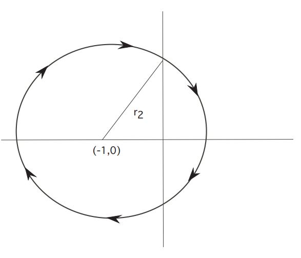

In summary, to get to the origin we must switch our control $\alpha (\cdot )$ back and forth between the values $\pm 1$, causing the trajectory to switch between lying on circles centered at $(\pm 1,0)$. The switches occur each π units of time.