8 Optimal Control with Differential-Algebraic Equations

So far we have regarded optimal control problems based on model dynamics in their simplest explicit-ODE form:

$$\dot{\mathit{x}}(t)=\mathit{f}(\mathit{x}(t),\mathit{\alpha }(t)).$$

This form of model for dynamic systems tend to arise naturally from the first-principle modelling approaches standardly taught and used by engineers. As a result, most continuous dynamic systems are described via explicit ODEs. It is a common but less widespread knowledge that for a large number of applications, building a dynamic model in the form of explicit ODEs can be significantly more involved and yield dramatically more complex model equations than via alternative model forms. Before laying down some theory, let us start with a simple illustrative example that we will use throughout this chapter.

Example 8.1

Consider a mass $m$ attached to a fixed point via a rigid link of length $L$ for which one wants to develop a dynamic model. A classic modelling approach is to describe the mass via two angles (azimuth and elevation of the mass), which yields an explicit ODE. The alternative model construction we will consider here describes the system via the cartesian coordinates $\mathit{p}\in {\mathbb{R}}^3$ of the mass in a fixed, inertial reference frame $E$ positioned at the attachment point of the mass, see Figure 8.1.

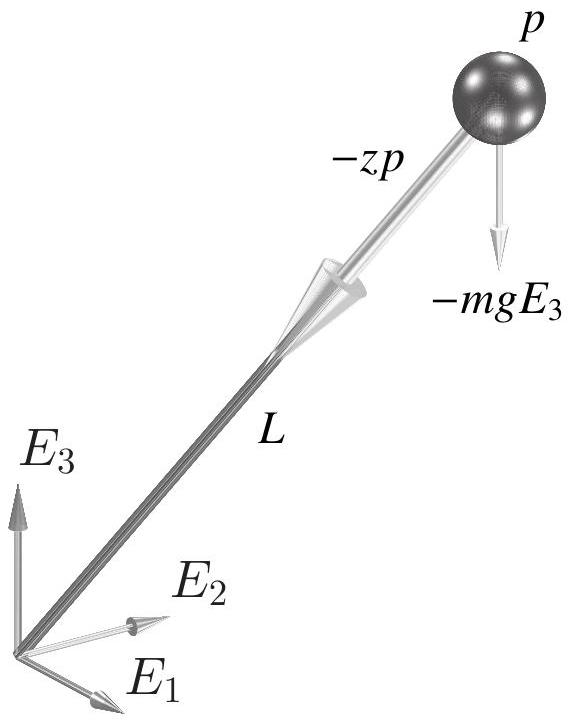
Figure 8.1: Illustration of the example considered in this chapter. The system is described via the cartesian position of the mass $\mathit{p}\in {\mathbb{R}}^3$ in the fixed frame $E$. The mass is subject to the gravity force $-mg{\mathit{E}}_3$ and to a force $-z\mathit{p}$ from the rod, which ensures that the mass remains at a distance $L$ from its attachment point. Here the scalar $z$ is a variable in the dynamics that scales this force adequately.

The rod maintains the mass at a distance $L$ of its attachment point by applying a force on the mass along its axis, i.e. having the support vector $\mathit{p}$. We will then describe the force of the $\mathrm{rod}$ as $F_{\text{rod }}=-z\mathit{p}$, where $z\in \mathbb{R}$ is a variable that adjusts the force magnitude to maintain the mass on a sphere of radius $L$, i.e. such that the condition ${\mathit{p}}^{\mathrm{\top }}\mathit{p}-L^2=0$ holds at all time. The model of the system can then takes a very simple form:

$$\begin{array}{}\text{(8.1)}& m\ddot{\mathit{p}}=\alpha -z\mathit{p}+mg{\mathit{E}}_3,\frac{1}{2}({\mathit{p}}^{\mathrm{\top }}\mathit{p}-L^2)=0.\end{array}$$

where ${\mathit{E}}_3^{\mathrm{\top }}=\left[\begin{array}{lll}0& 0& 1\end{array}\right]$. One can readily observe here that the model equation $(8.1)$ is not a simple explicit ODE. Indeed, while the scalar variable $z$ is intrinsically part of the model, its time derivative does not appear in the model equation. Hence, variable $z$ is of a different nature than variable $p$. A variable that is intrinsic to the model equation (i.e. excluding possibly time-varying parameters and inputs) but that is not time differentiated in the model equation is labelled an algebraic state. A differential equation holding such variables is called a Differential Algebraic Equation (DAE).

Following up on this example, we will now provide a more formal view on the concept of Differential-Algebraic Equations.

8.1 What are DAEs ?

Let us consider a differential equation in a very generic form:

$$\begin{array}{}\text{(8.2)}& \mathit{f}(\dot{\mathit{x}}(t),\mathit{x}(t),\mathit{\alpha }(t))=0.\end{array}$$

Such a differential equation is labelled implicit as the state derivative $\dot{x}(t)$ is not provided via an explicit function of the state $\mathit{x}(t)$ and input $\mathit{\alpha }(t)$, but implicitly as the solution of $(8.2)$.

The Implicit Function Theorem guarantees that $\dot{\mathit{x}}(t)$ can be seen as a locally unique and continuously differentiable function of $\mathit{x}(t)$ and $\mathit{\alpha }(t)$ if the Jacobian of $f$ with respect to $\dot{\mathit{x}}(t)$, i.e. $\frac{\partial f}{\partial \dot{\mathit{x}}}$, is full rank. Under this condition, one is guaranteed that for a given state $\mathit{x}(t)$ and input $\mathit{\alpha }(t)$, the state time derivative $\dot{\mathit{x}}(t)$ can be computed, either explicitly or numerically e.g. via a Newton iteration. Then $(8.2)$ is an Ordinary Differential Equation, since $\dot{\mathit{x}}(t)$ can be computed at every time instant, and the model can in principle be treated as a classic explicit ODE.

Formally, Differential-Algebraic Equations are equations in the form $(8.2)$ for which the above rank condition fails. Let us formalise that in the following definition.

Definition DAE

$\mathit{f}(\dot{\mathit{x}}(t),\mathit{x}(t),\mathit{\alpha }(t))=0$ is a DAE if $\frac{\partial \mathit{f}}{\partial \dot{\mathit{x}}}$ is rank deficient.

It is admittedly not straightforward to relate Definition above to the earlier example $(8.1)$. Before making this relationship clear, let us illustrate Definition above on a simple example.

Example 8.2

Let us consider the following implicit differential equation, having the form $(8.2)$:

$$\begin{array}{}\text{(8.3)}& f(\dot{x},x,\alpha )=\left[\begin{array}{c}{x}_1-{\dot{x}}_1+1\\ {\dot{x}}_1{x}_2+2\alpha \end{array}\right]=0,\end{array}$$

then the Jacobian of $f$ with respect to the state derivatives $\dot{x}$ reads as:

$$\frac{\partial f}{\partial \dot{x}}=\left[\begin{array}{cc}-1& 0\\ x_2& 0\end{array}\right]$$

and is rank-deficient, entailing that $(8.3)$ is, by Definition above, a DAE.

Alternatively, one can also simply observe that ${\dot{x}}_2$ does not appear time-differentiated in $(8.3)$, such that one can assess by simple inspection that it is a DAE.

In order to gain some further intuition in this example, consider solving the first equation in $(8.3)$ for ${\dot{x}}_1$, giving

$${\dot{x}}_1=x_1+1$$

Upon inserting the expression for ${\dot{x}}_1$ in the second equation, one can then write $(8.3)$ as

$$\begin{array}{rl}{\dot{x}}_1& =x_1+1,\\ 0& =(x_1+1)x_2+2.\end{array}$$

We observe here that the second equation is in fact purely algebraic, such that the model can be written as a mixture of an explicit differential equation and of an algebraic equation. This form of DAE is actually the most commonly used in practice. It is referred to as a semi-explicit DAE.

The above example can mislead one to believe that DAEs are fairly simple objects. To dispel that impression, let us provide a simple example of a DAE that possess fairly exotic properties.

Example 8.3

Let us consider the following differential equation

$$\begin{array}{rl}{\dot{x}}_1+x_1-\alpha & =0,\\ (x_1-x_2){\dot{x}}_2+x_1-x_2& =0,\end{array}$$

having the Jacobian

$$\frac{\partial f}{\partial \dot{x}}=\left[\begin{array}{cc}1& 0\\ 0& x_1-x_2\end{array}\right]$$

which is rank-deficient for $x_1=x_2$. Hence for the initial conditions:

$$x_1(0)=x_2(0)$$

our equation is a DAE and its solution obeys:

$$\begin{array}{rl}{\dot{x}}_1& =\alpha -x_1\\ 0& =x_2-x_1\end{array}$$

otherwise it is an ODE. The fact that some differential equation can switch between being DAEs and ODEs betrays the fact that DAEs are not necessarily simple to handle and analyse. However, in the context of numerical optimal control, simple DAEs are typically favoured.

About DAE

As observed before, DAEs often simply arise from the fact that some states in the state vector $x$ do not appear time-differentiated in the model equations, yielding a column of zeros in the Jacobian $\frac{\partial f}{\partial \dot{x}}$, as e.g. in example (8.2). In such a case, it is very useful to make an explicit distinction in the implicit differential equation (8.2) between the differential variables, i.e. the variables whose time derivative appear in $f$, typically labelled $x$, and the algebraic variables, i.e. the variables whose time derivative do not appear in $f$, typically labelled $z$. One can then rewrite (8.2) as:

$$\begin{array}{}\text{(8.4)}& \mathit{f}(\dot{\mathit{x}},\mathit{z},\mathit{x},\mathit{\alpha })=0.\end{array}$$

A DAE in the form $(8.4)$ is called a fully-implicit DAE. The application of definition of DAE to $(8.4)$ must then be understood in the sense that

$$\begin{array}{}\text{(8.5)}& \det \left(\begin{array}{cc}\frac{\partial f}{\partial \dot{x}}& \frac{\partial f}{\partial \dot{z}}\end{array}\right)=\det \left(\begin{array}{cc}\frac{\partial f}{\partial \dot{x}}& 0\end{array}\right)=0\end{array}$$

is always rank deficient. The differential equation $(8.4)$ is therefore always a DAE.

As mentioned in example 8.2, a common form of DAE often used in practice is the so-called semi-explicit form. It consists in explicitly splitting the DAE between an explicit differential equation and an implicit algebraic one. It reads as:

$$\begin{array}{rl}& \dot{x}=f(x,z,\alpha ),\\ & 0=g(x,z,\alpha ).\end{array}$$

The semi-explicit form is the most commonly used form of DAEs in optimal control. We turn next to a very important notion in the world of Differential-Algebraic Equations, both in theory and in practice.

8.2 Differential Index of DAEs

Before introducing the notion of differential index for DAE, it will be useful to take a brief and early tour into the problem of solving DAEs. Consider the semi-explicit DAE:

$$\begin{array}{}\text{(8.6a)}& & \dot{x}=f(x,z,\alpha ),\text{(8.6b)}& & 0=g(x,z,\alpha ),\end{array}$$

and suppose that one can construct (possibly via a numerical algorithm such as a Newton iteration) a function $\xi (x,\alpha )$ such that:

$$g(x,\xi (x,\alpha ),\alpha )=0,\mathrm{\forall }x,\alpha$$

That is, function $\xi (x,\alpha )$ delivers the algebraic state $z$ for any differential state $x$ and input $\alpha$. One can then proceed with eliminating the algebraic state $z$ in $(8.6)$, such that the DAE reads as:

$$\begin{array}{}\text{(8.7a)}& \dot{x}& =f(x,\xi (x,\alpha ),\alpha ),\text{(8.7b)}& z& =\xi (x,\alpha ).\end{array}$$

One can observe that $(8.7a)$ is then an explicit ODE, and can therefore be handled via any classical numerical integration method. Moreover, $(8.7b)$ provides the algebraic states explicitly. When such an elimination of the algebraic states is possible, one can consider the DAE $(8.6)$ as "easy" to solve.

It is then natural to ask when such an elimination is possible. The Implicit Function Theorem (IFT) provides here a straightforward answer, namely the function $\xi (x,\alpha )$ exists (locally) if the Jacobian

$$\begin{array}{}\text{(8.8)}& \frac{\partial }{\partial z}g(x,z,\alpha )\end{array}$$

is full rank along the trajectories $x,\alpha ,z$ of the system. The full-rankness of the Jacobian $(8.8)$ additionally guarantees that the Newton iteration:

$$\begin{array}{}\text{(8.9)}& z\leftarrow z-{\frac{\partial g(x,z,\alpha )}{\partial z}}^{-1}g(x,z,\alpha )\end{array}$$

converges locally to the solution $z$ of $(8.6b)$. In that sense, $(8.9)$ can be seen as a numerical procedure for constructing the implicit function $\xi (x,\alpha )$.

These notions easily extend to fully-implicit DAEs in the distinct form $(8.4)$. More specifically, suppose that there exists two functions ${\xi }_{\dot{x}}(x,\alpha )$ and ${\xi }_z(x,\alpha )$ that satisfy the fully implicit DAE $(8.4)$, i.e.

$$f({\xi }_{\dot{x}}(x,\alpha ),{\xi }_z(x,\alpha ),x,\alpha )=0,\mathrm{\forall }x,\alpha$$

Then one can rewrite $(8.4)$ as:

$$\begin{array}{}\text{(8.10a)}& \dot{x}& ={\xi }_{\dot{x}}(x,\alpha )\text{(8.10b)}& z& ={\xi }_z(x,\alpha ).\end{array}$$

Similarly to $(8.7)$, one can treat $(8.10a)$ as a simple ODE, while $(8.10b)$ delivers the algebraic states $z$ explicitly. The existence of functions ${\xi }_{\dot{x}}(x,\alpha )$ and ${\xi }_z(x,\alpha )$ can then again be guaranteed by invoking the IFT, namely if for $(8.4)$ the Jacobian matrix

$$\begin{array}{}\text{(8.11)}& \left[\begin{array}{ll}\frac{\partial f}{\partial \dot{x}}& \frac{\partial f}{\partial z}\end{array}\right]\end{array}$$

is full rank, then functions ${\xi }_{\dot{x}}(x,\alpha )$ and ${\xi }_z(x,\alpha )$ exist locally. The attentive reader will want to observe the important distinction between $(8.5)$ which always hold for $(8.4)$, and $(8.11)$ whose full-rankness guarantees the local existence of the implicit functions ${\xi }_{\dot{x}}(x,\alpha )$ and ${\xi }_z(x,\alpha )$.

Let us consider two examples to illustrate these notions.

Example 8.4

Consider again the fully-implicit DAE of Example 8.2, i.e.:

$$f(\dot{x},z,x,\alpha )=\left[\begin{array}{c}x-\dot{x}+1\\ \dot{x}z+2\end{array}\right]=0$$

We observe that

$$\left[\begin{array}{ll}\frac{\partial f}{\partial \dot{x}}& \frac{\partial f}{\partial z}\end{array}\right]=\left[\begin{array}{rr}-1& 0\\ z& \dot{x}\end{array}\right]$$

is full rank whenever $\dot{x}\ne 0$, such that the implicit functions ${\xi }_{\dot{x}}(x,\alpha )$ and ${\xi }_z(x,\alpha )$ are guaranteed to exist when $\dot{x}\ne 0$. In this simple case, they can actually be computed explicitly. Indeed, we observe that:

$$\dot{x}={\xi }_{\dot{x}}(x,\alpha )=x+1,z={\xi }_z(x,\alpha )=-\frac{2}{x+1}$$

solve $f(\dot{x},z,x,\alpha )$ whenever $\dot{x}=x+1\ne 0$.

This simple example needs to be pitted against a more problematic one.

Example 8.5

Consider the fully-implicit DAE:

$$\mathit{f}(\dot{\mathit{x}},z,\mathit{x},\alpha )=\left[\begin{array}{c}{\dot{x}}_1-z\\ {\dot{x}}_2-x_1\\ x_2-\alpha \end{array}\right]=0$$

We observe that:

$$\left[\begin{array}{ll}\frac{\partial \mathit{f}}{\partial \dot{\mathit{x}}}& \frac{\partial \mathit{f}}{\partial z}\end{array}\right]=\left[\begin{array}{ccc}1& 0& -1\\ 0& 1& 0\\ 0& 0& 0\end{array}\right]$$

is always rank-deficient, such that the differential state $\dot{\mathit{x}}$ and algebraic state $z$ cannot be uniquely obtained (even numerically) from solving $f(\dot{\mathit{x}},z,\mathit{x},\alpha )=0$ alone.

differential index

The topic of this section is the notion of differential index of DAEs. As we will see next, the loose idea of "easy" DAEs presented above is directly related to it. Let us introduce now the notion of differential index for DAEs.

Definition: differential index of a DAE

The differential index of a DAE is the number of times it must be time-differentiated before an explicit ODE is obtained.

For the specific case of a semi-explicit DAE, the above definition also reads as follows.

Definition: differential index of the semi-explicit DAE

The differential index of the semi-explicit DAE $(8.6)$ is the number of times its algebraic part $(8.6b)$ must be time-differentiated before an explicit ODE is obtained.

In order to clarify these definitions, let us make a simple example.

Example 8.5

Let us calculate the differential index of the DAE proposed in Example 8.2, i.e.:

$$f(\dot{x},z,x)=\left[\begin{array}{c}x-\dot{x}+1\\ \dot{x}z+2\end{array}\right]=0$$

We then consider the time derivative of $f$, i.e.:

$$\begin{array}{}\text{(8.12)}& \dot{f}(\ddot{x},\dot{x},x,\dot{z},z)=\left[\begin{array}{c}\dot{x}-\ddot{x}\\ \ddot{x}z+\dot{x}\dot{z}\end{array}\right]=0.\end{array}$$

For the sake of clarity, we label $\mathit{v}=\left[\begin{array}{c}x\\ z\\ \dot{x}\end{array}\right]$ and rewrite (8.12) in the equivalent form:

$$\mathit{\zeta }(\dot{\mathit{v}},\mathit{v})=\left[\begin{array}{c}{\dot{v}}_1-v_3\\ v_3-{\dot{v}}_3\\ {\dot{v}}_3{v}_2+v_3{\dot{v}}_2\end{array}\right]=0$$

The Jacobian

$$\frac{\partial \mathit{\zeta }(\dot{v},v)}{\partial \dot{v}}=\left[\begin{array}{ccc}1& 0& 0\\ 0& 0& -1\\ 0& v_3& v_2\end{array}\right]$$

is then full rank, such that $\mathit{\zeta }$ is an ODE for $\mathit{v}$ according to Definition of DAE. Since a single time-differentiation has converted the original DAE of this example into an ODE, we can conclude that the original DAE is of index $1$.

Let us contrast this example with a DAE having a higher differential index.

Example 8.6

Let us calculate the differential index of our illustrative example $(8.1)$. Using $v=\dot{p}$, and defining the differential state vector

$$x=\left[\begin{array}{l}p\\ v\end{array}\right]$$

one can easily verify that the DAE $(8.1)$ can be written as a semi-explicit DAE:

$$\begin{array}{}\text{(8.13a)}& \dot{p}& =v,\text{(8.13b)}& \dot{v}& =m^{-1}\alpha -m^{-1}zp+g{E}_3,\text{(8.13c)}& 0& =\underset{=g(x,z,\alpha )}{\underbrace{\frac{1}{2}(p^{\mathrm{\top }}p-L^2)}}.\end{array}$$

We observe that for a given $z$, $(8.13a)-(8.13b)$ are already ODEs in $v$ and $p$. As per Definition of differential index of semi-explicit DAE, we need to differentiate the algebraic equation $(8.13c)$ until $(8.13)$ becomes an ODE. The two first time derivatives read as:

$$\dot{g}(x,z,\alpha )=p^{\mathrm{\top }}v=0,\text{ and }\ddot{g}(\dot{x},x,z,\alpha )=p^{\mathrm{\top }}\dot{v}+v^{\mathrm{\top }}v=0$$

One can then use $(8.13b)$ in $\ddot{g}(\dot{x},x,z,\alpha )$ to obtain

$$\ddot{g}(\dot{x},x,z,\alpha )=p^{\mathrm{\top }}(\alpha -m^{-1}zp+g{E}_3)+v^{\mathrm{\top }}v=0$$

As $z$ now appears explicitly in $\ddot{g}(\dot{x},x,z,\alpha )$, an extra time-differentiation yields a differential equation from which $\dot{z}$ can be computed if $p^{\mathrm{\top }}p\ne 0$. We observe that $3$ time-differentiations of $(8.13c)$ were necessary to turn $(8.13)$ into an ODE. It follows that $(8.13)$ is an index-$3$ DAE.

index $1$ DAE

Now we ought to relate the notion of "easy" DAEs to the notion of differential index. More specifically, we shall see next that index-1 DAEs are "easy" DAEs in the sense detailed previously. This observation can be formally described in the following Lemma.

Lemma

For any fully-implicit index-$1$ DAE

$$f(\dot{x},z,x,\alpha )=0$$

there exists implicit functions ${\xi }_{\dot{x}}(x,\alpha )$ and ${\xi }_z(x,\alpha )$ that satisfy:

$$f({\xi }_{\dot{x}}(x,\alpha ),{\xi }_z(x,\alpha ),x,\alpha )=0,\mathrm{\forall }x,\alpha .$$

Proof: We observe that if $f$ is of index 1 , then a single time-differentiation:

$$\dot{f}=\frac{\partial f}{\partial \dot{x}}\ddot{x}+\frac{\partial f}{\partial z}\dot{z}+\frac{\partial f}{\partial x}\dot{x}+\frac{\partial f}{\partial \alpha }\dot{\alpha }=0$$

yields a pure ODE. For the sake of clarity, we label $v=\left[\begin{array}{c}\dot{x}\\ z\end{array}\right]$ and write:

$$\begin{array}{}\text{(8.14)}& \dot{f}=\left[\begin{array}{ll}\frac{\partial f}{\partial \dot{x}}& \frac{\partial f}{\partial z}\end{array}\right]\dot{v}+\frac{\partial f}{\partial x}\dot{x}+\frac{\partial f}{\partial \alpha }\dot{\alpha }=0.\end{array}$$

By assumption, $(8.14)$ can be written as an explicit ODE, hence $\left[\begin{array}{ll}\frac{\partial f}{\partial \dot{x}}& \frac{\partial f}{\partial z}\end{array}\right]$ must be full rank, such that:

$$\dot{v}=-{\left[\begin{array}{ll}\frac{\partial f}{\partial \dot{x}}& \frac{\partial f}{\partial z}\end{array}\right]}^{-1}(\frac{\partial f}{\partial x}\dot{x}+\frac{\partial f}{\partial \alpha }\dot{\alpha })$$

holds on the DAE trajectories. The IFT then guarantees the existence of the implicit functions ${\xi }_{\dot{x}}(x,\alpha )$ and ${\xi }_z(x,\alpha )$ in a neighborhood of the trajectories of the DAE.

$◻$

A similar result can clearly be established for any index-$1$ semi-explicit DAEs on the existence of an implicit function ${\xi }_z(x,\alpha )$ that solves the algebraic equation, i.e. such that

$$g(x,{\xi }_z(x,\alpha ),\alpha )=0,\mathrm{\forall }x,\alpha$$

The crucial practical consequence of these observations is that index-$1$ DAEs can be in principle solved numerically (or sometimes even explicitly) without difficulties, as for any state and input $x(t)$ and $\mathit{\alpha }(t)$, the state derivative $\dot{x}(t)$ and algebraic state $z(t)$ can be computed, and the simulation of the dynamics performed. In practice, implicit integration methods are the most efficient approach to perform the simulations of index-$1$ DAEs, while DAEs of index higher than $1$ require specially-tailored integrators.

A non-trivial but important point needs to be stressed here. DAEs of index higher than $1$ , often labelled high-index DAEs, present a pitfall to uninformed users of numerical methods. Indeed, one deploying a classical implicit integration method on a high-index DAE may observe that the implicit integration method converges reliably and be mislead into believing that simulations of the DAE model can be reliably computed. In order to clarify this issue, let us consider the following example, based on a linear, high-index DAE.

Example 8.7

In this example, we are interested to observe the result of "naively" deploying a classical implicit integration scheme on a high-index DAE. We consider again the fully-implicit DAE of Example 8.5, i.e.

$$\begin{array}{}\text{(8.15)}& f(\dot{x},z,x,\alpha )=\left[\begin{array}{c}{\dot{x}}_1-z\\ {\dot{x}}_2-x_1\\ x_2-\alpha \end{array}\right]\end{array}$$

The reader can easily verify that $(8.15)$ is not an index-$1$ DAE. We observe that we can rewrite $(8.15)$ in the linear form $E\dot{v}=Av+B\alpha$, where

$$\mathit{v}=\left[\begin{array}{l}x\\ z\end{array}\right],E=\left[\begin{array}{lll}1& 0& 0\\ 0& 1& 0\\ 0& 0& 0\end{array}\right],A=\left[\begin{array}{ccc}0& 0& 1\\ 1& 0& 0\\ 0& -1& 0\end{array}\right],\mathit{B}=\left[\begin{array}{l}0\\ 0\\ 1\end{array}\right].$$

We are interested now in naively deploying an implicit Euler scheme of step length $h$ on this DAE, yielding the steps:

$$\frac{1}{h}E({\mathit{v}}_{+}-\mathit{v}(t))=A{\mathit{v}}_{+}+\mathit{B}\mathit{\alpha }(t+h)$$

where ${\mathit{v}}_{+}$is an approximation of the state at time $\mathit{v}(t+h)$, i.e. ${\mathit{v}}_{+}\approx \mathit{v}(t+h)$. It can be verified that the true trajectories $\mathit{v}(t+h)$ satisfy:

$$E[\frac{1}{h}(\mathit{v}(t+h)-\mathit{v}(t))+\frac{h}{2}\ddot{x}(\tau )]=A\mathit{v}(t+h)+\mathit{B}\mathit{\alpha }(t+h)$$

for some $\tau \in [t,t+h]$. We can then consider the one-step integration error ${\mathit{e}}_{+}={\mathit{v}}_{+}-\mathit{v}(t+h)$ given by:

$${\mathit{e}}_{+}=\frac{{\mathit{h}}^2}{2}(E-A\mathit{h}{)}^{-1}E\ddot{\mathit{x}}(\tau ).$$

For DAE $(8.15)$, matrix $\frac{h^2}{2}(E-Ah{)}^{-1}E$ reads as:

$$\frac{h^2}{2}(E-Ah{)}^{-1}E=\frac{1}{2}\left[\begin{array}{lll}0& h& 0\\ 0& 0& 0\\ h& 1& 0\end{array}\right],$$

such that the integration error is of order $\mathcal{O}(1)$, i.e. much worse than the integration error expected from the implicit Euler method, which is of order $\mathcal{O}\left(h^2\right)$.

This simple example reveals that, even though a classic implicit integration scheme deployed on high-index DAEs $(8.15)$ can in some cases reliably deliver state trajectories, their lousy numerical accuracy typically makes them actually meaningless as simulations of the DAE model. The difficulty with DAE $(8.15)$ stems from its index larger than 1 . These observations must be taken as a warning that while one can sometimes deploy a classical implicit integration scheme on a high-index DAE without observing notable numerical difficulties, the resulting trajectories are typically nonetheless senseless. Hence, good practice in numerical optimization dictates that the index of a DAE ought to be systematically checked before tackling it via classical integration methods.

Because index-$1$ DAEs are significantly easier to treat than high-index DAEs, it is common in numerical optimal control to avoid DAEs of index larger than $1$. Unfortunately, the index of a DAE stems from the nature of the physical system it models and cannot be decided. However, a treatment of high-index DAEs generally allows one to ultimately treat them as index-$1$ DAEs. We will cover this question next.

8.3 Index reduction

As detailed in the previous Section, index-$1$ DAEs are simpler to treat numerically than high-index DAEs, as index-$1$ DAEs can be approached using standard implicit integration methods. This observation motivates the deployment of procedures for reducing the index of an arbitrary high-index DAE into an index-$1$ DAE, a procedure labelled index reduction. Index-reduction proceeds very similarly to the procedure leading to assess the index of a DAE, i.e. via time-differentiation of the DAE (or of some parts of the DAE) until a DAE of index $1$ is obtained. In order to explain this further, let us detail it on our illustrative example $(8.1)$.

Example 8.8

We consider again the semi-explicit DAE $(8.13)$, i.e.

$$\begin{array}{}\text{(8.16a)}& \dot{\mathit{p}}& =\mathit{v},\text{(8.16b)}& \dot{\mathit{v}}& =\alpha -m^{-1}z\mathit{p}+g{\mathit{E}}_3,\text{(8.16c)}& 0& =\underset{=g(x,z,\alpha )}{\underbrace{\frac{1}{2}({\mathit{p}}^{\mathrm{\top }}\mathit{p}-L^2)}},\end{array}$$

which is in a semi-explicit form. Similarly to the index evaluation presented in Example 8.6, i.e. we consider the time-derivatives of the algebraic equation (8.16c)

$$\dot{g}(x,z,\alpha )=p^{\mathrm{\top }}v=0,\text{ and }\ddot{g}(\dot{x},x,z,\alpha )=p^{\mathrm{\top }}\dot{v}+v^{\mathrm{\top }}v=0$$

One can then easily verify that the new DAE:

$$\begin{array}{}\text{(8.17a)}& \dot{\mathit{p}}& =\mathit{v},\text{(8.17b)}& m\dot{\mathit{v}}& =\alpha -z\mathit{p}+mg{\mathit{E}}_3,\text{(8.17c)}& 0& =\underset{=\ddot{g}(\dot{x},x,z,\alpha )}{\underbrace{{\mathit{p}}^{\mathrm{\top }}\dot{\mathit{v}}+{\mathit{v}}^{\mathrm{\top }}\mathit{v}}},\end{array}$$

is of index $1$. Alternatively, it is useful to put $(8.17)$ in a more implicit form:

$$\begin{array}{}\text{(8.18a)}& \dot{\mathit{p}}& =\mathit{v},\text{(8.18b)}& \left[\begin{array}{ll}m& \mathit{p}\\ {\mathit{p}}^{\mathrm{\top }}& 0\end{array}\right]\left[\begin{array}{l}\dot{\mathit{v}}\\ \mathit{z}\end{array}\right]& =\left[\begin{array}{c}\alpha +mg{\mathit{E}}_3\\ -{\mathit{v}}^{\mathrm{\top }}\mathit{v}\end{array}\right],\end{array}$$

which shows unambiguously that the state derivatives $\dot{\mathit{v}}$ and $\dot{\mathit{p}}$ as well as the algebraic state $z$ can be computed for any state $\mathit{v},\mathit{p}$ and input $\alpha$ as long as $\mathit{p}\ne 0$. This observation tells us without further investigation that (8.18) is an "easy" DAE, i.e. of index $1$.

Index-reduction procedures can be fairly intricate to deploy on very complex models. For the sake of completeness, let us report here a recipe for performing the index-reduction on any semi-explicit DAE:

$$\begin{array}{rl}& \dot{x}=f(x,z,\alpha )\\ & 0=g(x,z,\alpha )\end{array}$$

1. Check if the DAE system is index $1$ (i.e. $\frac{\partial g}{\partial z}$ full rank). If yes, stop.
2. Identify a subset of algebraic equations that can be solved for a subset of algebraic variables.
3. Perform a time-differentiation on the remaining algebraic equations that contain (some of) the differential variables $x$. Terms $\dot{x}$ will appear in these differentiated equations.
4. Substitute the $\dot{x}$ with their corresponding symbolic expressions $f(x,z,\alpha )$. This generates new algebraic equations.
5. With this new DAE system, go to step 1.

Our discussion on index reduction would not complete if we omit the question of consistency conditions. To understand this issue, consider the indexreduced DAE developed in Example 8.8, which takes the form:

$$\begin{array}{}\text{(8.19a)}& \dot{x}& =f(x,z,\alpha )\text{(8.19b)}& 0& =\ddot{g}(\dot{x},x,z,\alpha )\end{array}$$

One needs to observe here that while a solution to the original DAE $(8.16)$ in the form

$$\begin{array}{}\text{(8.20a)}& & \dot{x}=f(x,z,\alpha )\text{(8.20b)}& & 0=g(x,z,\alpha )\end{array}$$

is obviously also a solution for the index-reduced DAE (8.19), the converse is not necessarily true, i.e. a solution of the index-reduced DAE $(8.19)$ is not necessarily a solution to the original DAE $(8.20)$. To understand this statement, one simply ought to imagine a trajectory that is solution of $(8.19a)$, and for which

$$\begin{array}{}\text{(8.21)}& g(x(t),z(t),\mathit{\alpha }(t))=g(x(0),z(0),\mathit{\alpha }(0))+t\dot{g}(x(0),z(0),\mathit{\alpha }(0))=0\end{array}$$

holds. This trajectory clearly satisfies $(8.19b)$ but not $(8.20b)$. Equation $(8.21) $additionally reveals that the issue is not related the DAEs themselves, but rather to the initial conditions chosen for the simulation of the DAEs. Indeed, simply selecting the initial conditions $x(0)$ such that

$$\begin{array}{}\text{(8.22)}& g(x(0),z(0),\mathit{\alpha }(0))=0,\text{ and }\dot{g}(x(0),z(0),\mathit{\alpha }(0))=0\end{array}$$

ensures that the trajectories of the index-reduced DAE are solution of the original one. More generally, enforcing

$$\begin{array}{}\text{(8.23)}& g(x\left(t_0\right),z\left(t_0\right),\alpha \left(t_0\right))=0,\text{ and }\dot{g}(x\left(t_0\right),z\left(t_0\right),\alpha \left(t_0\right))\end{array}$$

at any time $t_0$ on the trajectory guarantees a simulation run with the indexreduced DAE is a valid simulation of the original DAE. Conditions that guarantees the validity of the simulation performed on the index-reduced DAE, such as $(8.23)$, are labelled consistency conditions.

In the context of optimal control based on an index-reduced DAE, consistency conditions are crucial when the trajectories of the differential states of system do not have (fully) prescribed initial or terminal values. In such a case, the consistency conditions must be adequately enforced within the optimal control problem. E.g. an optimal control problem involving our index-reduced DAE $(8.18)$ having free initial or terminal states can e.g. be written as:

$$\begin{array}{}\text{(8.24)}& \begin{array}{rlrlrl}\underset{\mathit{v},\mathit{p},z,\alpha }{\min }& {\int }_0^{T}g(\mathit{v},\mathit{p},z,\alpha )\mathrm{d}t& & & & \\ \text{ subject to }& \dot{\mathit{p}}=\mathit{v}& & \text{ (Differential equ.), }\\ & m\dot{\mathit{v}}=\alpha -z\mathit{p}+mg{\mathit{E}}_3& & \text{ (Differential equ.), }\\ & 0={\mathit{p}}^{\mathrm{\top }}\dot{\mathit{v}}+{\mathit{v}}^{\mathrm{\top }}\mathit{v}& & \text{(Algebratic equ.), }\\ & 0=\mathit{p}{\left(t_0\right)}^{\mathrm{\top }}\mathit{v}\left(t_0\right)& & \text{ (Consistency cond.), }\\ & 0=\mathit{p}{\left(t_0\right)}^{\mathrm{\top }}\dot{\mathit{v}}\left(t_0\right)+\mathit{v}{\left(t_0\right)}^{\mathrm{\top }}\mathit{v}\left(t_0\right)& & \text{ (Consistency cond.) }\end{array}\end{array}$$

for any $t_0\in [0,T]$.

It ought to be underlined here that imposing some constraints on the initial and/or terminal state trajectories in conjunction with imposing the consistency conditions must be done with great care in order to avoid generating a redundant set of constraints in the OCP. As a trivial example of this difficulty, imposing e.g. the initial states in $(8.24)$ in addition to the consistency conditions with $t_0=0$ would clearly over-constrain the initial state values $\mathit{p}(0),\mathit{v}(0)$. This issue can become significantly more involved in less obvious scenarios, such as e.g. in periodic OCPs, where the initial and terminal states are free but must satisfy a periodicity constraint of the form $x(0)=x(T)$. Handling the consistency conditions and the periodicity constraints together in the OCP without generating an over-constrained problem can then become fairly involved.

The consistency conditions can in principle be enforced at any time $t_0$ in the time span considered by the OCP. However, in some cases the selection of the time $t_0$ for imposing the consistency condition is not arbitrary. Indeed, one ought to observe that the combination of the index-reduced algebraic constraint and of the consistency conditions, i.e.

$$\begin{array}{}\text{(8.25)}& \ddot{g}(x(t),z(t),\mathit{\alpha }(t))& =0\text{(8.26)}& \dot{g}(x\left(t_0\right),z\left(t_0\right),\alpha \left(t_0\right))& =0\text{(8.27)}& g(x\left(t_0\right),z\left(t_0\right),\alpha \left(t_0\right))& =0\end{array}$$

ensure mathematically that

$$g(x(t),z(t),\mathit{\alpha }(t))=g(x\left(t_0\right),z\left(t_0\right),\alpha \left(t_0\right))+(t-t_0)\dot{g}(x\left(t_0\right),z\left(t_0\right),\alpha \left(t_0\right))=0$$

holds at any time $t$. However, when the DAE dynamics are handled via numerical integration, numerical errors tend to accumulate over time such that $g(x(t),z(t),\mathit{\alpha }(t))=0$ can be less accurately enforced at times that are distant from $t_0$. From this observation one ought to conclude that if the solution to an OCP is e.g. more important at the beginning of the time span the OCP covers, say $[0,T]$, then the consistency conditions ought to be enforced in the beginning of the time span, i.e. $t_0=0$. This situation occurs in Nonlinear Model Predictive Control (NMPC), where the first control input $q_0$ delivered by the OCP provides the control input to be deployed on the real system, such that the accuracy of the solution in the beginning of the time interval it covers is the more important than later in the horizon.

Conversely, if the OCP implements a Moving Horizon Estimation (MHE) scheme, then the differential state obtained at the very end of the time span covered by the OCP delivers a state estimation to e.g. an NMPC scheme. In such a case, the accuracy is most important at the very end of the time interval, such that the consistency conditions are best imposed at $t_0=T$.

8.4 Direct Methods with Differential-Algebraic Equations

We will now turn to discussing the deployment of direct optimal control methods on OCPs involving DAEs. For the reasons detailed previously, we will focus on OCPs involving index-$1$ DAEs, possibly arising from an index-reduction of a high-index DAE.

8.4.1 Numerical Solution of Differential-Algebraic Equations

In this Section, we will briefly discuss the numerical solution of DAEs. As hinted above, index-$1$ DAEs are significantly simpler to treat numerically than high-index ones, and are therefore often preferred in optimal control. In this Section, we will focus in the index-$1$ case.

Though low-order methods generally offer a poor ratio between accuracy and computational complexity and higher-order integrators should be preferred, let use nonetheless start here with a simple $m$-step implicit Euler scheme for the sake of illustration. For e.g. a semi-explicit DAE

$$\begin{array}{rl}& \dot{x}=f(x,z,\alpha ),\\ & 0=g(x,z,\alpha ),\end{array}$$

the $m$-step implicit Euler scheme computes a numerical simulation $x(t_{k+1},{\beta }_k,q_k)$ of the model dynamics over a time interval $[t_k,t_{k+1}]$ from the initial state ${\beta }_k$ and the constant input $q_k$ via the following algorithm.

Algorithm 8.13 (Implicit Euler integrator). Input: initial value ${\beta }_k$, input $q_k$ and times $t_k,t_{k+1}$ Set $v=q_k$, and $h=(t_{k+1}-t_k)/m$for $i=0$ to $m-1$ do Solve

$$\begin{array}{rl}{x}_{+}& =v+hf(x_{+},z_{+},q_k)\\ 0& =g(x_{+},z_{+},q_k)\end{array}$$

for $x_{+},z_{+}$via a Newton iteration, set $v\leftarrow x_{+}$. end forOutput: $x(t_{k+1},{\beta }_k,q_k)=v$

A similar approach can be deployed using any implicit integration method, such as an IRK4 integrator.

A fairly efficient and useful type of implicit integrator already introduced in Section 7.3 is the orthogonal collocation approach. Let us consider the building of the collocation equations for DAEs in a generic implicit form

$$\begin{array}{}\text{(8.29)}& f(\dot{x},x,z,\alpha )=0\end{array}$$

on a time interval $[t_k,t_{k+1}]$, with initial value ${\beta }_k$ and a constant input $q_k$. The differential states are, as in the ODE case described via polynomials $p(t,v_k)$, with $t\in [t_k,t_{k+1}]$ linearly parametrized in $v_k$ such that:

• the polynomial interpolation meets the initial value, i.e.:

$$\begin{array}{}\text{(8.30)}& \underset{=v_{k,0}}{\underbrace{p(t_k,v_k)}}={\beta }_k\end{array}$$

• the DAE is satisfied in the collocation times $t_{k,i}$ for $i=1,\dots ,d$, i.e.:

$$\begin{array}{}\text{(8.31)}& f({\dot{p}}_k(t_{k,i},v_k),\underset{=v_{k,i}}{\underbrace{p_k(t_{k,i},v_k)}},z_{k,i},q_k)=0,i=1,\dots ,d\end{array}$$

We can gather these requirements in the compact implicit equation:

$$\begin{array}{}\text{(8.32)}& c_k(v_k,z_k,q_k,{\beta }_k)=\left[\begin{array}{c}{v}_{k,0}-{\beta }_k\\ f({\dot{p}}_k(t_{k,1},v_k),v_{k,1},z_{k,1},q_k)\\ ⋮\\ f({\dot{p}}_k(t_{k,d},v_k),v_{k,d},z_{k,d},q_k)\end{array}\right]=0.\end{array}$$

The same observations as for the semi-explicit case hold for the general case.

One ought to observe that the discretized algebraic states $z_{k,i}$ appear only for the indices $i=1,\dots ,d$ in the collocation equations, while the discretized differential states $v_{k,i}$ appear for the indices $i=0,\dots ,d$. I.e. the discrete algebraic states $z_k$ have one DoF less that the discrete differential states $v_k$. The extra DoF granted to the differential state is actually required in order to be able to meet the initial value ${\beta }_k$ of the differential state trajectories, while the initial value of algebraic state trajectories cannot be assigned as they are already defined implicitly by the DAE, subject to the imposed state initial value ${\beta }_k$ and input $q_k$. This observation is most obvious in the semi-explicit case, where for a given state initial value ${\beta }_k$ and input $q_k$, the initial value for the algebraic state is implicitly given by $g({\beta }_k,z\left(t_k\right),q_k)=0$.

For the sake of completeness, let us provide the algorithm for a collocation-based integrator for index-$1$ DAEs.

Algorithm 8.14 (Collocation-based integrator). Input: initial value ${\beta }_k$ input $q_k$, initial guess $v_k,z_k$ and times $t_k,t_{k+1}$ Solve

$$\begin{array}{}\text{(8.33)}& c_k(v_k,z_k,q_k,{\beta }_k)=0\end{array}$$

for $v_k,z_k$ via a Newton iteration Output: $x(t_{k+1},{\beta }_k,q_k)=p_k(t_{k+1},v_k)$

It is interesting to observe here that while the algorithm ought to receive an initial guess for the discrete algebraic states $z_k$, it receives an initial value ${\beta }_k$ only for the differential state. It is also important to notice that the algebraic states $z_k$ can in principle be entirely hidden inside the integrator (even though they can be, of course, reported).

Sensitivities of the integrators

The computation of the sensitivities of an implicit integrator such as $(8.14)$ can be done as detailed in Section 10.4(in referenced e-books). More specifically, if we label ${\mathit{w}}_k=\left[\begin{array}{l}{v}_k\\ z_k\end{array}\right]$, the collocation equation $(8.36)$ in algorithm $8.14$ is typically solved using a (often full-step) Newton iteration:

$$\begin{array}{}\text{(8.34)}& {\mathit{w}}_k={\mathit{w}}_k-\frac{\partial c_k{({\mathit{w}}_k,q_k,{\beta }_k)}^{-1}}{\partial {\mathit{w}}_k}{c}_k({\mathit{w}}_k,q_k,{\beta }_k)\end{array}$$

The sensitivities are then provided at the solution $c_k({\mathit{w}}_k,q_k,{\beta }_k)=0$ by:

$$\begin{array}{}\text{(8.35a)}& & \frac{\partial {\mathit{w}}_k}{\partial q_k}=-\frac{\partial c_k{({\mathit{w}}_k,q_k,{\beta }_k)}^{-1}}{\partial {\mathit{w}}_k}\frac{\partial c_k({\mathit{w}}_k,q_k,{\beta }_k)}{\partial q_k}\text{(8.35b)}& & \frac{\partial {\mathit{w}}_k}{\partial {\beta }_k}=-\frac{\partial c_k{({\mathit{w}}_k,q_k,{\beta }_k)}^{-1}}{\partial {\mathit{w}}_k}\frac{\partial c_k({\mathit{w}}_k,q_k,{\beta }_k)}{\partial {\beta }_k}\end{array}$$

It is important to note here that a factorization of the Jacobian matrix $\frac{\partial c_k({\mathit{w}}_k,q_k,{\beta }_k)}{\partial {\mathit{w}}_k}$ is already computed for the Newton iterations $(8.34)$ and the last factorization can be readily reused at the end of the iteration to form the sensitivities $(8.35)$. The computational complexity of obtaining the sensitivities consists then only of the computation of the matrices $\frac{\partial c_k({\mathit{w}}_k,q_k,{\beta }_k)}{\partial {\beta }_k}$ and $\frac{\partial c_k({\mathit{w}}_k,q_k,{\beta }_k)}{\partial q_k}$ and the matrix products in $(8.35)$. A collocation-based integrator with sensitivities then reads as:

Algorithm 8.15 (Collocation-based integrator with Sensitivities). Input: initial value ${\beta }_k$ input $q_k$, initial guess $v_k,z_k$ and times $t_k,t_{k+1}$ Solve

$$\begin{array}{}\text{(8.36)}& c_k(v_k,z_k,q_k,{\beta }_k)=0\end{array}$$

for $v_k,z_k$ via a Newton iteration Compute $(8.35)$ Form:

$$\begin{array}{}\text{(8.37)}& & \frac{\partial x(t_{k+1},{\beta }_k,q_k)}{\partial {\beta }_k}=\frac{\partial p_k(t_{k+1},v_k)}{\partial v_k}\frac{\partial v_k}{\partial {\mathit{w}}_k}\frac{\partial {\mathit{w}}_k}{\partial {\beta }_k}\text{(8.38)}& & \frac{\partial x(t_{k+1},{\beta }_k,q_k)}{\partial q_k}=\frac{\partial p_k(t_{k+1},v_k)}{\partial v_k}\frac{\partial v_k}{\partial {\mathit{w}}_k}\frac{\partial {\mathit{w}}_k}{\partial q_k}\end{array}$$

Output: $x(t_{k+1},{\beta }_k,q_k)=p_k(t_{k+1},v_k)$, and $\frac{\partial x(t_{k+1},{\beta }_k,q_k)}{\partial {\beta }_k},\frac{\partial x(t_{k+1},{\beta }_k,q_k)}{\partial q_k}$ where $\frac{\partial v_k}{\partial {\mathit{w}}_k}=\left[\begin{array}{ll}I& 0\end{array}\right]$ is constant.

We can now turn to the deployment of Multiple-Shooting on DAE-based optimal control problems.

8.4.2 Direct Multiple-Shooting with Differential-Algebraic Equations

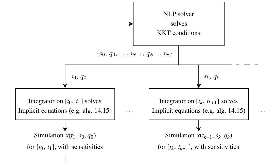
Figure 8.4.1: The diagram

In the context of Multiple-Shooting for DAE-based optimal control problems, the implicit numerical integration schemes detailed above are interacting with the NLP solver tackling the NLP resulting from the Multiple-Shooting discretization. We illustrate this interaction in Figure above. The NLP solver is then responsible for closing the shooting gaps, i.e. enforcing the continuity conditions:

$$x(t_{k+1},{\beta }_k,q_k)-{\beta }_{k+1}=0$$

for $k=0,\dots ,N-1$, and solving the set of algebraic equations that capture the conditions of optimality. It is interesting to observe here that the overall process can be then construed as a "two-level Newton scheme", where the upper level solve the KKT conditions (e.g. using the relaxed KKT obtained in the primal-dual interior-point approach, or using SQP iterations) and the lower level solves the equations underlying the numerical integration (e.g. $(8.36)$). The NLP solver passes the discrete states and inputs ${\beta }_k,q_k$, which become inputs to the numerical integration algorithms, while the numerical integration algorithms report to the NLP solver the end states of the simulations $x(t_{k+1},{\beta }_k,q_k)$ and their sensitivities.

One ought to observe here that the algebraic state dynamics can in principle be totally "hidden" inside the integrator scheme, and not reported at all to the NLP solver. In that sense, implicit integrators in general perform an elimination of the algebraic variables present in the dynamics, and hide their existence to the NLP solver.

Another crucial observation to make here is that no continuity condition nor initial condition is enforced on the algebraic state trajectories $z(t)$. Indeed, for a given differential state trajectory $x(t)$ and input profile $\mathit{\alpha }(t)$, the algebraic state trajectories $z(t)$ are entirely defined via the DAE (e.g. by $g(x,z,\alpha )=0$ in the semi-explicit case), such that an extra continuity condition imposed on $z(t)$ would yield an over-constrained problem. As a matter of fact, if a discontinuous input parametrization is used (such as e.g. piecewise-constant), the algebraic state trajectories $z(t)$ can be discontinuous at the time instants $t_k$ corresponding to the multiple-shooting time grid. E.g. in the semi-explicit case and if the algebraic equation $g(x,z,\alpha )=0$ depends on $\alpha$, at the time instants $t_k$, a discontinuous input typically requires $z(t)$ to also be discontinuous.

As mentioned previously, the integrator can hide the algebraic variables from the NLP solvers and keep them as purely internal. However, one may want to use these variables in the cost function of the OCP, or impose some inequality constraints on them. In such a case, the algebraic states ought to be reported to the NLP solver, where they are regarded as functions of the decision variables ${\beta }_k,q_k$.

As illustrated in Figure 8.4.1, Multiple-Shooting with implicit integrators can be viewed as a two-level Newton scheme, where algebraic conditions are solved at two different levels. A natural alternative to this setup is then clearly to introduce the algebraic conditions underlying the numerical integrators into the NLP, and leave them to be solved by the NLP solver. Doing so leads us back to the Direct Collocation scheme, which we revisit next in the context of DAE-based optimal control problems.

8.4.3 Direct Collocation with Differential-Algebraic Equations

We will focus now on the deployment of the Direct Collocation method on such DAE-based optimal control problems. The principle here is extremely similar to those detailed in Section 7.3. However, there are a few important additional specific details arising from the presence of algebraic states and equations that need to be properly covered here. Let us briefly recall here the core principles of the direct collocation method. As detailed earlier in Section 7.3 and briefly recalled in Section 8.4.1 above, the differential state trajectories are approximated on each time intervals $[t_k,t_{k+1}]$ via the polynomials $p_k(t,v_k)$ linearly parametrized by the set of variables $v_k\in {\mathbb{R}}^{n(d+1)}$. For an explicit ODE $\dot{x}=f(x,\alpha )$, the collocation equations then enforce:

• the continuity conditions of the differential states at the times $t_k$ for $k=0,\dots ,N-1$

$$\begin{array}{}\text{(8.39)}& p_k(t_{k+1},v_k)-{\beta }_{k+1,0}=0,\end{array}$$

• the state dynamics at the times $t_{k,i}$ for $k=0,\dots ,N-1$ and $i=1,\dots ,d$

$${\dot{p}}_k(t_{k,i},v_k)=f(v_{k,i},q_k)$$

Additional conditions are typically added as boundary conditions, e.g. $v_{0,0}-x_0=0$ to enforce the initial condition of the state trajectories.

The extension of the collocation equations for a semi-explicit DAE

$$\begin{array}{rl}& \dot{x}=f(x,z,\alpha )\\ & 0=g(x,z,\alpha )\end{array}$$

follow the exact same philosophy, namely the collocation equations enforce:

• the continuity conditions of the differential states via $(8.39)$ at the times $t_{0,\dots ,N-1}$.
• the state dynamics at the times $t_{k,i}$ for $k=0,\dots ,N-1$ and $i=1,\dots ,d$ via

$$\begin{array}{}\text{(8.40a)}& {\dot{p}}_k(t_{k,i},v_k)& =f(v_{k,i},z_{k,i},q_k)\text{(8.40b)}& 0& =g(v_{k,i},z_{k,i},q_k)\end{array}$$

The collocation equations for a semi-implicit DAE therefore read as:

$$\begin{array}{}\text{(8.41)}& c_k(v_k,z_k,q_k,v_{k+1})=\left[\begin{array}{c}{\dot{p}}_k(t_{k,1},v_k)-f(v_{k,1},q_k)\\ g(v_{k,1},z_{k,1},q_k)\\ ⋮\\ {\dot{p}}_k(t_{k,d},v_k)-f(v_{k,d},q_k)\\ g(v_{k,d},z_{k,d},q_k)\\ p_k(t_{k+1},v_k)-v_{k+1,0}\end{array}\right]=0.\end{array}$$

for $k=0,\dots ,N-1$.

A few details ought to be properly stressed here.

1. similarly to the observations made in Section 8.4.2, no continuity condition is enforced on the algebraic states, hence $(8.39)$ applies to the differential state trajectories alone.
2. one ought to observe that the discretized algebraic states $z_{k,i}$ appear only for the indices $i=1,\dots ,d$ in the collocation equations, i.e. the discrete algebraic states have one DoF less that the discrete differential states $v_{k,i}$ which appear with the indices $i=0,\dots ,d$ in the collocation equations. The extra DoF granted to the differential state is actually required in order to be able to impose the continuity of the differential state trajectories, while the algebraic state trajectories are not required to be continuous. When building the NLP arising from a discretization of a DAE-based OCP using direct collocation, one ought to make sure that the adequate number of discrete algebraic states and discrete differential states are declared to the NLP solver. Indeed, e.g. introducing by mistake the unnecessary extra variables $z_{k,0}$ can create numerical difficulties in the solver, as these variables would be "free" in the NLP and their values not clearly fixed by the problem.

Building the collocation equations for DAEs in a generic implicit form

$$f(\dot{x},x,z,u)=0$$

is a natural generalization of the constraints used in the case of a semi-explicit DAE. In the general case, the collocation equations simply read as:

$$c_k(v_k,z_k,q_k,v_{k+1})=\left[\begin{array}{c}f({\dot{p}}_k(t_{k,1},v_k),v_{k,1},z_{k,1},q_k)\\ ⋮\\ f({\dot{p}}_k(t_{k,d},v_k),v_{k,d},z_{k,1},q_k)\\ p_k(t_{k+1},v_k)-v_{k+1,0}\end{array}\right]=0$$

for $k=0,\dots ,N-1$. The same observations as for the semi-explicit case hold for the general case.