1 Introduction

Reference e-book: An Introduction to Mathematical Optimal Control Theory by Lawrence C. Evans in 2024

1.1 basic problem

DYNAMICS: Consider an ODE:

$$\{\begin{array}{rl}\dot{\mathit{x}}(t)& =\mathit{f}(\mathit{x}(t))(t>0)\\ \mathit{x}(0)& =x^0\end{array}$$

• $x^0\in {\mathbb{R}}^n$: initial point
• $\mathit{f}:{\mathbb{R}}^n\to {\mathbb{R}}^n$: dynamic function
• $\mathit{x}:[0,\mathrm{\infty })\to {\mathbb{R}}^n$: unknown; dynamic evolution of the state of some "system"

CONTROLLED DYNAMICS: Generalize a bit, $\mathit{f}$ also depends upon some "control" parameters $a\in A\subset {\mathbb{R}}^m$. So $\mathit{f}:{\mathbb{R}}^n\times A\to {\mathbb{R}}^n$:

$$\{\begin{array}{rl}\dot{\mathit{x}}(t)& =\mathit{f}(\mathit{x}(t),a)(t>0)\\ \mathit{x}(0)& =x^0\end{array}$$

Change the value $a$ as the system evolves, like:

$$\mathit{\alpha }(t)=\{\begin{array}{ll}{a}_1& 0\le t\le t_1\\ a_2& t_1<t\le t_2\\ a_3& t_2<t\le t_3\end{array}etc.$$

Then the dynamic equation becomes:

$$\{\begin{array}{rl}\dot{\mathit{x}}(t)& =\mathit{f}(\mathit{x}(t),\mathit{\alpha }(t))(t>0)\\ \mathit{x}(0)& =x^0\end{array}$$

We call a function $\mathit{\alpha }:[0,\mathrm{\infty })\to A$ a control and regard the trajectory $\mathit{x}(t)$ as te corresponding response of the system.

Notation

• Introduce:

  $$\mathcal{A}=\{\mathit{\alpha }:[0,\mathrm{\infty })\to A|\mathit{\alpha }(\cdot )\mathrm{measurable}\}$$

  To denote the collection of all admissible controls

• $\mathit{x}(\cdot )=\mathit{x}(\cdot ,\mathit{\alpha }(\cdot ),x^0)$ would be more precise

Payoffs

Overall task will be to determine what is the "best" control for our system. For this we need to specify a specific payoff (or reward) criterion. Let us define the payoff functional

$$P[\mathit{\alpha }(\cdot )]:={\int }_0^{T}r(\mathit{x}(t),\mathit{\alpha }(t))\mathrm{d}t+g(\mathit{x}(T))$$

where:

• $\mathit{x}(\cdot )$ solves ODE for the control $\mathit{\alpha }(\cdot )$
• $r:{\mathbb{R}}^n\times A\to \mathbb{R}$: Given; runnig payoff
• $g:{\mathbb{R}}^n\to \mathbb{R}$: Given; terminal payoff;
• $T$: Given; terminal time

The basic problem

Aim: find a control ${\mathit{\alpha }}^{\ast }(\cdot )$ which maximizes the payoff:

$$P[{\mathit{\alpha }}^{\ast }(\cdot )]\ge P[\mathit{\alpha }(\cdot )].$$

for all controls $\mathit{\alpha }(\cdot )\in \mathcal{A}$. Such a control ${\mathit{\alpha }}^{\ast }(\cdot )$ is called an optimal control.

This task presents us with these mathematical issues:

1. Does an optimal control exist?
2. How can we characterize an optimal control mathematically?
3. How can we construct an optimal control?

These turn out to be sometimes subtle problems, as the following collection of examples illustrates.

1.2 Examples

Example 1: Control of Production and Consumption

Suppose we own, say, a factory whose output we can control. Let us begin to construct a mathematical model by setting

$x(t)=$ amount of output produced at time $t\ge 0$

We suppose that we consume some fraction of our output at each time, and likewise can reinvest the remaining fraction. Let us denote:

$\alpha (t)=$ fraction of output reinvested at time $t\ge 0$

This will be our control, and s.t. the obvious constraint that:

$$0\le \alpha (t)\le 1,\text{for each time }t\ge 0$$

The corresponding dynamic equation is:

$$\{\begin{array}{rl}\dot{x}(t)& =k\alpha (t)x(t)(t>0)\\ x(0)& =x^0\end{array}$$

The constant $k>0$ modelling the growth rate of our reinvestment.

Take as a payoff functional:

$$P[\alpha (\cdot )]:={\int }_0^T(1-\alpha (t))x(t)\mathrm{d}t$$

That means we want to maximize our total consumption of the output, our consumption at a given time t being $(1-\alpha (t))x(t)$. Here $n=m=1$ and:

$$A=[0,1],f(x,a)=kax,r(x,a)=(1-a)x,g\equiv 0.$$

In 4.4.2, we will see that the optimal control is ${\alpha }^{\ast }$ is given by:

$${\alpha }^{\ast }=\{\begin{array}{ll}1& 0\le x(t)\le t^{\ast }\\ 0& t^{\ast }<x(t)\le T\end{array}$$

In other words, we should reinvest all the output (and therefore consume nothing) up until time $t^{\ast }$, and afterwards, we should consume everything (and therefore reinvest nothing). The switchover time $t^{\ast }$ will have to be determined. We call ${\alpha }^{\ast }(\cdot )$ a bang–bang control.

Example 2: Reproduction Strategies in Social Insects

In this example, we consider a population of social insects, a population if bees. Write $T$ for the length of the season,, and introduce the variables:

• $w(t)=$ number of workers at time $t$
• $q(t)=$ number of queens
• $\alpha (t)=$ fraction of colony effort devoted to increasing work force

Constraint of $\alpha (t)$: $0\le \alpha (t)\le 1$

Introduce the dynamic for the numbers of workers and the number of queens:

• workers:$$\{\begin{array}{rl}\dot{w}(t)& =-\mu w(t)+bs(t)\alpha (t)w(t)\\ w(0)& =w^0\end{array}$$
  • $\mu$:is the death rate of workers; given constant
  • $s(t)$: the known rate at which each worker contributes to the bee economy
• queens:$$\{\begin{array}{rl}\dot{q}(t)& =-\nu q(t)+c(1-\alpha (t))s(t)w(t)\\ q(0)& =q^0\end{array}$$
  • $\nu ,c$ constant

Goal: maximize the queens at time $T$:

$$P[\alpha (\cdot )]=q(T)$$

We have $\mathit{x}(t)=(w(t),q(t){)}^{\mathrm{\top }}$ and $x^0=(w^0,q^0{)}^{\mathrm{\top }}$, take $r\equiv 0$ and $g(w,q)=q$

answer will again turn out to be a bang–bang control

Example 3: A Pendulum

A hanging pendlum: $\theta (t)=$ angle of the pendulum at time $t\ge 0$

If no external force:

$$\{\begin{array}{rl}& \ddot{\theta }(t)+\lambda \dot{\theta }(t)+{\omega }^2\theta (t)=0\\ & \theta (0)={\theta }_1,\dot{\theta }(0)={\theta }_2\end{array}$$

The solution will be a damped oscillation, provided $\lambda >0$

Let $\alpha (t)$ denote an applied torque: $|\alpha |\le 1$

Our dynamics now become

$$\{\begin{array}{l}\ddot{\theta }(t)+\lambda \dot{\theta }(t)+{\omega }^2\theta (t)=\alpha (t)\\ \theta (0)={\theta }_1,\dot{\theta }(0)={\theta }_2\end{array}$$

Define $x_1(t)=\theta (t),x_2(t)=\dot{\theta }(t)$, and $\mathit{x}(t)=(x_1(t),x_2(t))$. Then we can write the evolution as the system

$$\dot{\mathit{x}}(t)=(\genfrac{}{}{0ex}{}{{\dot{x}}_1}{{\dot{x}}_2})=(\genfrac{}{}{0ex}{}{\dot{\theta }}{\ddot{\theta }})=(\genfrac{}{}{0ex}{}{x_2}{-\lambda x_2-{\omega }^2{x}_1+\alpha (t)})=\mathit{f}(\mathit{x},\alpha ).$$

We introduce as well

$$P[\alpha (\cdot )]=-{\int }_0^{\tau }1dt=-\tau$$

for

$$\tau =\tau (\alpha (\cdot ))=\text{ first time that }\mathit{x}(\tau )=0\text{ (that is, }\theta (\tau )=\dot{\theta }(\tau )=0.)$$

Maximize $P[\cdot ]$, meaning that we want to minimize the time it takes to bring the pendulum to rest.

The terminal time isn't fixed, but rather depends upon the control. This's a fixed endpoint, free time problem.

Example 4: A Moon Lander

This model asks us to bring a spacecraft to a soft landing on the lunar surface, using the least amount of fuel.

Introduce the notation:

Notation

• $h(t)$: height at time $t$
• $v(t)$: velocity $=\dot{h}(t)$
• $m(t)$: mass of spacecraft at time $t$ (changing as fuel is burned)
• $\alpha (t)$: thrust at time t, assumed that $0\le \alpha (t)\le 1$

For Newton's law:

$$m\ddot{h}=-gm+\alpha$$

Modelled by ODE:

$$\{\begin{array}{rl}\dot{v}(t)& =-g+\frac{\alpha (t)}{m(t)}\\ \dot{h}(t)& =v(t)\\ \dot{m}(t)& =-k\alpha (t)\end{array}$$

We want to minimize the amount of fuel used up, that is, to maximize the amount remaining once we have landed. Thus

$$P[\alpha (\cdot )]=m(\tau )$$

where $\tau$ is the first time that $h(\tau )=v(\tau )=0$. This's a variable endpoint problem, since the final time is not given in advance.

We have also the extra constraints $h(t)\ge 0,m(t)\ge 0$

Example 5: Rocket Railroad Car

Imagine a railroad car powered by rocket engines on each side. We introduce the variables:

• $q(t)$: position at time $t$
• $v(t)=\dot{q}(t)$: velocity at time $t$
• $\alpha (t)$: thrust from rockets at time $t$, assumed that $-1\le \alpha (t)\le 1$

We want to figure out how to fire the rockets, so as to arrive at the origin 0 with zero velocity in a minimum amount of time. Assuming the car has mass $m=1$, the law of motion is

$$\ddot{q}(t)=\alpha (t)$$

Rewrie by setting $\mathit{x}(t)=(q(t),v(t){)}^{\mathrm{\top }}$. Then

$$\{\begin{array}{l}\dot{\mathit{x}}(t)=\left(\begin{array}{ll}0& 1\\ 0& 0\end{array}\right)\mathit{x}(t)+(\genfrac{}{}{0ex}{}{0}{1})\alpha (t)\\ \mathit{x}(0)=x^0={(q_0,v_0)}^T\end{array}$$

Take

$$P[\alpha (\cdot )]=-{\int }_0^{\tau }1\mathrm{d}t=-\tau$$

for $\tau =$ first time that $q(\tau )=v(\tau )=0$

1.3 A geometric solution

Introduce some ad hoc calculus and geometry methods for the rocke car problem.

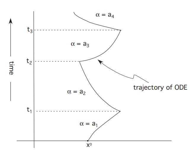
First of all, let us guess that to find an optimal solution we will need only to consider the cases $\alpha =1$ or $\alpha =-1$. In other words, we will focus our attention only upon those controls for which at each moment of time either the left or the right rocket engine is fired at full power.

• CASE 1: $\alpha \equiv 1$

  $$\{\begin{array}{l}\dot{q}=v\\ \dot{v}=1\end{array}$$

  Then

  $$v\dot{v}=\dot{q}$$

  And so

  $$\frac{1}{2}(v^2{)}^{\cdot }=\dot{q}$$

  Let $t_0$ belong to the time interval where $\alpha \equiv 1$ and interate from $t_0$ to $t$:

  $$\frac{v^2(t)}{2}-\frac{v^2(t_0)}{2}=q(t)-q(t_0)$$

  Then

  $$v^2(t)=2q(t)+\underset{b}{\underbrace{(v^2\left(t_0\right)-2q\left(t_0\right))}}$$

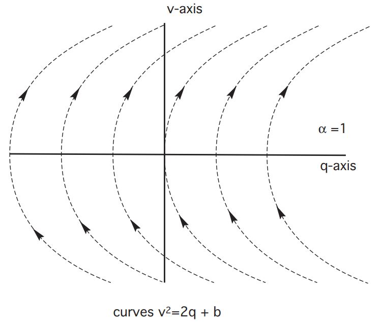
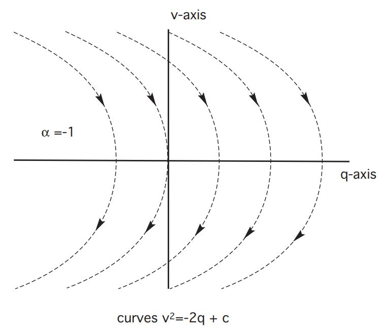
  In other words, so long as the control is set for $\alpha \equiv 1$, the trajectory stays on the curve $v^2=2q+b$ for some constant $b$.

  

• CASE 2: $\alpha \equiv -1$

  $$\{\begin{array}{l}\dot{q}=v\\ \dot{v}=-1\end{array}$$

Then

$$\frac{1}{2}(v^2{)}^{\cdot }=-\dot{q}$$

Let $t_1$ belong to the time interval where $\alpha \equiv -1$ and interate from $t_1$ to $t$:

$$v^2(t)=-2q(t)+\underset{c}{\underbrace{(2q\left(t_1\right)-v^2\left(t_1\right))}}$$

As long as the control is set for $\alpha \equiv -1$, the trajectory stays on the curve $v^2=-2q+c$ for some constant $c$.

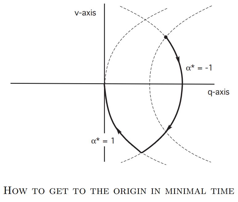
Geometric interpretation

Now we can design an optimal control ${\alpha }^{\ast }(\cdot )$, which causes the trajectory to jump between the families of right– and left–pointing parabolas, as drawn. Say we start at the black dot, and wish to steer to the origin. This we accomplish by first setting the control to the value $\alpha =-1$, causing us to move down along the second family of parabolas. We then switch to the control $\alpha =1$, and thereupon move to a parabola from the first family, along which we move up and to the left, ending up at the origin. See the picture.