5 Dynamic Programming

5.1 Derivation of Bellman's PDE

5.1.1 Dynamic Programming

We begin with some mathematical wisdom:

“It is sometimes easier to solve a problem by embedding it within a larger class of problems and then solving the larger class all at once.”

A Calculus Example

Suppose we wish to calculate the value of the integral

$${\int }_0^{\mathrm{\infty }}\frac{\sin x}{x}\mathrm{d}x$$

This is pretty hard to do directly, so let us as follows add a parameter $\alpha$ into the integral:

$$I(\alpha ):={\int }_0^{\mathrm{\infty }}{e}^{-\alpha x}\frac{\sin x}{x}\mathrm{d}x$$

We compute

$$I^{\prime }(\alpha )={\int }_0^{\mathrm{\infty }}(-x)e^{-\alpha x}\frac{\sin x}{x}\mathrm{d}x=-{\int }_0^{\mathrm{\infty }}\sin x{e}^{-\alpha x}\mathrm{d}x=-\frac{1}{{\alpha }^2+1}$$

where we integrated by parts twice to find the last equality. Consequently

$$I(\alpha )=-\arctan \alpha +C$$

and we must compute the constant $C$. To do so, observe that

$$0=I(\mathrm{\infty })=-\arctan (\mathrm{\infty })+C=-\frac{\pi }{2}+C,$$

and so $C=\frac{\pi }{2}$. Hence $I(\alpha )=-\arctan \alpha +\frac{\pi }{2}$, and consequently

$${\int }_0^{\mathrm{\infty }}\frac{\sin x}{x}\mathrm{d}x=I(0)=\frac{\pi }{2}$$

Come back to control

We want to adapt some version of this idea to the vastly more complicated setting of control theory. For this, fix a terminal time $T>0$ and then look at the controlled dynamics

$$\begin{array}{}\text{(ODE)}& \{\begin{array}{l}\dot{\mathit{x}}(s)=\mathit{f}(\mathit{x}(s),\mathit{\alpha }(s))\\ \mathit{x}(0)=x^0,\end{array}\end{array}$$

with the associated payoff functional

$$\begin{array}{}\text{(P)}& P[\mathit{\alpha }(\cdot )]={\int }_0^{T}r(\mathit{x}(s),\mathit{\alpha }(s))\mathrm{d}s+g(\mathit{x}(T)).\end{array}$$

We embed this into a larger family of similar problems, by varying the starting times and starting points:

$$\begin{array}{}\text{(5.1)}& \{\begin{array}{ll}\dot{\mathit{x}}(s)=\mathit{f}(\mathit{x}(s),\mathit{\alpha }(s))& (t\le s\le T)\\ \mathit{x}(t)=x.& \end{array}\end{array}$$

with

$$\begin{array}{}\text{(5.2)}& P_{x,t}[\mathit{\alpha }(\cdot )]={\int }_t^{T}r(\mathit{x}(s),\mathit{\alpha }(s))\mathrm{d}s+g(\mathit{x}(T)).\end{array}$$

Consider the above problems for all choices of starting times $0\le t\le T$ and all initial points $x\in {\mathbb{R}}^n$.

Definition: value function

For $x\in {\mathbb{R}}^n,0\le t\le T$, define the value function $v(x,t)$ to be the greatest payoff possible if we start at $x\in {\mathbb{R}}^n$ at time $t$. In other words,

$$\begin{array}{}\text{(5.3)}& v(x,t):=\underset{\mathit{\alpha }(\cdot )\in \mathcal{A}}{sup}{P}_{x,t}[\mathit{\alpha }(\cdot )](x\in {\mathbb{R}}^n,0\le t\le T).\end{array}$$

Notice then that

$$\begin{array}{}\text{(5.4)}& v(x,T)=g(x)(x\in {\mathbb{R}}^n).\end{array}$$

5.1.2 Derivation of Hamilton-Jacobi-Bellman Equation

Our first task is to show that the value function $v$ satisfies a certain nonlinear partial differential equation.

Our derivation will be based upon the reasonable principle that

"it's better to be smart from the beginning, than to be stupid for a time and then become smart".

We want to convert this philosophy of life into mathematics.

To simplify, we hereafter suppose that the set $A$ of control parameter values is compact.

Theorem 5.1 (Hamilton-Jacobi-Bellman Equation)

Assume that the value function $v$ is a $C^1$ function of the variables ( $x,t$ ). Then $v$ solves the nonlinear partial differential equation

$$\begin{array}{}\text{(HJB)}& v_t(x,t)+\underset{a\in A}{max}\{\mathit{f}(x,a)\cdot {\mathrm{\nabla }}_{x}v(x,t)+r(x,a)\}=0(x\in {\mathbb{R}}^n,0\le t<T),\end{array}$$

with the terminal condition

$$v(x,T)=g(x)(x\in {\mathbb{R}}^n)$$

Remark

We call $(\mathrm{HJB})$ the Hamilton-Jacobi-Bellman equation, and can rewrite it as

$$\begin{array}{}\text{(HJB)}& v_t(x,t)+H(x,{\mathrm{\nabla }}_{x}v)=0(x\in {\mathbb{R}}^n,0\le t<T),\end{array}$$

for the partial differential equations Hamiltonian

$$H(x,p):=\underset{a\in A}{max}H(x,p,a)=\underset{a\in A}{max}\{\mathit{f}(x,a)\cdot p+r(x,a)\}$$

where $x,p\in {\mathbb{R}}^n$.

Proof

1. Let $x\in {\mathbb{R}}^n,0\le t<T$ and let $h>0$ be given. As always

$$\mathcal{A}=\{\mathit{\alpha }(\cdot ):[0,\mathrm{\infty })\to A\text{ measurable }\}.$$

Pick any parameter $a\in A$ and use the constant control

$$\mathit{\alpha }(\cdot )\equiv a$$

for times $t\le s\le t+h$. The dynamics then arrive at the point $\mathit{x}(t+h)$, where $t+h<T$. Suppose now a time $t+h$, we switch to an optimal control and use it for the remaining times $t+h\le s\le T$.

What is the payoff of this procedure? Now for times $t\le s\le t+h$, we have

$$\{\begin{array}{l}\dot{\mathit{x}}(s)=\mathit{f}(\mathit{x}(s),a)\\ \mathit{x}(t)=x\end{array}$$

The payoff for this time period is ${\int }_t^{t+h}r(\mathit{x}(s),a)\mathrm{d}s$. Furthermore, the payoff incurred from time $t+h$ to $T$ is $v(\mathit{x}(t+h),t+h)$, according to the definition of the payoff function $v$. Hence the total payoff is

$${\int }_t^{t+h}r(\mathit{x}(s),a)\mathrm{d}s+v(\mathit{x}(t+h),t+h)$$

But the greatest possible payoff if we start from ( $x,t$ ) is $v(x,t)$. Therefore

$$\begin{array}{}\text{(5.5)}& v(x,t)\ge {\int }_t^{t+h}r(\mathit{x}(s),a)\mathrm{d}s+v(\mathit{x}(t+h),t+h).\end{array}$$

2. We now want to convert this inequality into a differential form. So we rearrange $(5.5)$ and divide by $h>0$ :

$$\frac{v(\mathit{x}(t+h),t+h)-v(x,t)}{h}+\frac{1}{h}{\int }_t^{t+h}r(\mathit{x}(s),a)\mathrm{d}s\le 0$$

Let $h\to 0$ :

$$v_t(x,t)+{\mathrm{\nabla }}_{x}v(\mathit{x}(t),t)\cdot \dot{\mathit{x}}(t)+r(\mathit{x}(t),a)\le 0$$

But $\mathit{x}(\cdot )$ solves the ODE

$$\{\begin{array}{l}\dot{\mathit{x}}(s)=\mathit{f}(\mathit{x}(s),a)(t\le s\le t+h)\\ \mathit{x}(t)=x.\end{array}$$

Employ this above, to discover:

$$v_t(x,t)+\mathit{f}(x,a)\cdot {\mathrm{\nabla }}_{x}v(x,t)+r(x,a)\le 0.$$

This inequality holds for all control parameters $a\in A$, and consequently

$$\begin{array}{}\text{(5.6)}& \underset{a\in A}{max}\{v_t(x,t)+\mathit{f}(x,a)\cdot {\mathrm{\nabla }}_{x}v(x,t)+r(x,a)\}\le 0.\end{array}$$

3. We next demonstrate that in fact the maximum above equals zero. To see this, suppose ${\mathit{\alpha }}^{\ast }(\cdot ),{\mathit{x}}^{\ast }(\cdot )$ were optimal for the problem above. Let us utilize the optimal control ${\mathit{\alpha }}^{\ast }(\cdot )$ for $t\le s\le t+h$. The payoff is

$${\int }_t^{t+h}r({\mathit{x}}^{\ast }(s),{\mathit{\alpha }}^{\ast }(s))\mathrm{d}s$$

and the remaining payoff is $v({\mathit{x}}^{\ast }(t+h),t+h)$. Consequently, the total payoff is

$${\int }_t^{t+h}r({\mathit{x}}^{\ast }(s),{\mathit{\alpha }}^{\ast }(s))\mathrm{d}s+v({\mathit{x}}^{\ast }(t+h),t+h)=v(x,t).$$

Rearrange and divide by $h$ :

$$\frac{v({\mathit{x}}^{\ast }(t+h),t+h)-v(x,t)}{h}+\frac{1}{h}{\int }_t^{t+h}r({\mathit{x}}^{\ast }(s),{\mathit{\alpha }}^{\ast }(s))\mathrm{d}s=0.$$

Let $h\to 0$ and suppose ${\mathit{\alpha }}^{\ast }(t)=a^{\ast }\in A$. Then

$$v_t(x,t)+{\mathrm{\nabla }}_{x}v(x,t)\cdot \underset{\mathit{f}(x,a^{\ast })}{\underbrace{{\dot{\mathit{x}}}^{\ast }(t)}}+r(x,a^{\ast })=0;$$

and therefore

$$v_t(x,t)+\mathit{f}(x,a^{\ast })\cdot {\mathrm{\nabla }}_{x}v(x,t)+r(x,a^{\ast })=0$$

for some parameter value $a^{\ast }\in A$. This proves $(\mathrm{HJB})$.

$◻$

5.1.2 The Dynamic Programming Method

Here is how to use the dynamic programming method to design optimal controls:

Step 1: Solve the Hamilton-Jacobi-Bellman equation, and thereby compute the value function $v$.

Step 2: Use the value function $v$ and the Hamilton-Jacobi-Bellman PDE to design an optimal feedback control ${\mathit{\alpha }}^{\ast }(\cdot )$, as follows. Define for each point $x\in {\mathbb{R}}^n$ and each time $0\le t\le T$,

$$\mathit{\alpha }(x,t)=a\in A$$

to be a parameter value where the maximum in (HJB) is attained. In other words, we select $\mathit{\alpha }(x,t)$ so that

$$v_t(x,t)+\mathit{f}(x,\mathit{\alpha }(x,t))\cdot {\mathrm{\nabla }}_{x}v(x,t)+r(x,\mathit{\alpha }(x,t))=0.$$

Next we solve the following ODE, assuming $\mathit{\alpha }(\cdot ,t)$ is sufficiently regular to let us do so:

$$\begin{array}{}\text{(ODE)}& \{\begin{array}{l}{\dot{\mathit{x}}}^{\ast }(s)=\mathit{f}({\mathit{x}}^{\ast }(s),\mathit{\alpha }({\mathit{x}}^{\ast }(s),s))(t\le s\le T)\\ \mathit{x}(t)=x.\end{array}\end{array}$$

Finally, define the feedback control

$$\begin{array}{}\text{(5.7)}& {\mathit{\alpha }}^{\ast }(s):=\mathit{\alpha }({\mathit{x}}^{\ast }(s),s).\end{array}$$

In summary, we design the optimal control this way: If the state of system is $x$ at time $t$, use the control which at time $t$ takes on the parameter value $a\in A$ such that the minimum(fault, maximum?) in (HJB) is obtained.

We demonstrate next that this construction does indeed provide us with an optimal control.

Theorem 5.2 (Verification of Optimality)

The control ${\mathit{\alpha }}^{\ast }(\cdot )$ defined by the construction $(5.7)$ is optimal.

Proof of Theorem 5.2

We have

$$P_{x,t}[{\mathit{\alpha }}^{\ast }(\cdot )]={\int }_t^{T}r({\mathit{x}}^{\ast }(s),{\mathit{\alpha }}^{\ast }(s))\mathrm{d}s+g({\mathit{x}}^{\ast }(T)).$$

Furthermore according to the definition $(5.7)$ of $\mathit{\alpha }(\cdot )$ :

$$\begin{array}{rl}{P}_{x,t}[{\mathit{\alpha }}^{\ast }(\cdot )]& ={\int }_t^T(-v_t({\mathit{x}}^{\ast }(s),s)-\mathit{f}({\mathit{x}}^{\ast }(s),{\mathit{\alpha }}^{\ast }(s))\cdot {\mathrm{\nabla }}_{x}v({\mathit{x}}^{\ast }(s),s))\mathrm{d}s+g({\mathit{x}}^{\ast }(T))\\ & =-{\int }_t^T{v}_t({\mathit{x}}^{\ast }(s),s)+{\mathrm{\nabla }}_{x}v({\mathit{x}}^{\ast }(s),s)\cdot {\dot{\mathit{x}}}^{\ast }(s)\mathrm{d}s+g({\mathit{x}}^{\ast }(T))\\ & =-{\int }_t^T\frac{\mathrm{d}}{\mathrm{d}s}v({\mathit{x}}^{\ast }(s),s)\mathrm{d}s+g({\mathit{x}}^{\ast }(T))(ChainRule)\\ & =-v({\mathit{x}}^{\ast }(T),T)+v({\mathit{x}}^{\ast }(t),t)+g({\mathit{x}}^{\ast }(T))\\ & =-g({\mathit{x}}^{\ast }(T))+v({\mathit{x}}^{\ast }(t),t)+g({\mathit{x}}^{\ast }(T))\\ & =v(x,t)=\underset{\mathit{\alpha }(\cdot )\in \mathcal{A}}{sup}{P}_{x,t}[\mathit{\alpha }(\cdot )].\end{array}$$

That is,

$$P_{x,t}[{\mathit{\alpha }}^{\ast }(\cdot )]=\underset{\mathit{\alpha }(\cdot )\in \mathcal{A}}{sup}{P}_{x,t}[\mathit{\alpha }(\cdot )];$$

and so ${\mathit{\alpha }}^{\ast }(\cdot )$ is optimal, as asserted.

$◻$

5.2 Examples

5.2.1 Example 1: Dynamics with Three Velocities

Let us begin with a fairly easy problem:

$$\begin{array}{}\text{(ODE)}& \{\begin{array}{l}\dot{x}(s)=\alpha (s)(0\le t\le s\le 1)\\ x(t)=x\end{array}\end{array}$$

where our set of control parameters is

$$A=\{-1,0,1\}.$$

We want to minimize

$${\int }_t^1|x(s)|\mathrm{d}s$$

and so take for our payoff functional

$$\begin{array}{}\text{(P)}& P_{x,t}[\alpha (\cdot )]=-{\int }_t^1|x(s)|\mathrm{d}s.\end{array}$$

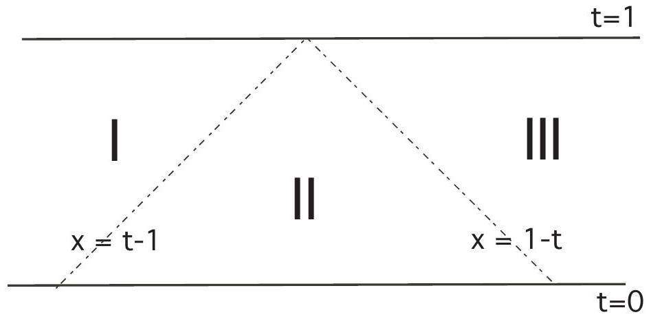
As our first illustration of dynamic programming, we will compute the value function $v(x,t)$ and confirm that it does indeed solve the appropriate Hamilton-Jacobi-Bellman equation. To do this, we first introduce the three regions:

• Region $I=\{(x,t)\mid x<t-1,0\le t\le 1\}$.
• Region $II=\{(x,t)\mid t-1<x<1-t,0\le t\le 1\}$.
• Region $III=\{(x,t)\mid x>1-t,0\le t\le 1\}$.

We will consider the three cases as to which region the initial data ( $x,t$ ) lie within.

• Region III

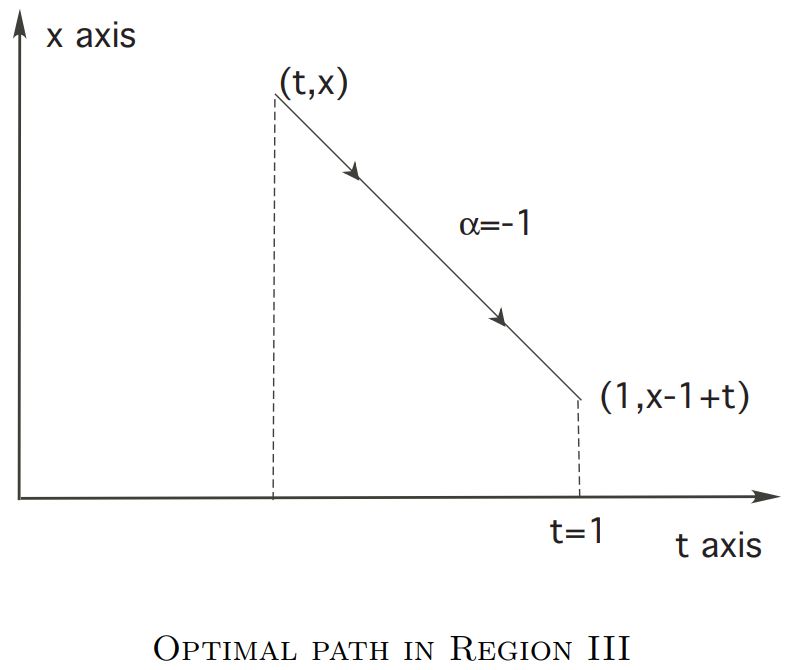
In this case we should take $\alpha \equiv -1$, to steer as close to the origin 0 as quickly as possible. Then

$$\begin{array}{rl}v(x,t)& =-\text{area under path taken}\\ & =-(1-t)\frac{1}{2}(x+x+t-1)=-\frac{(1-t)}{2}(2x+t-1).\end{array}$$

• Region I In this region, we should take $\alpha \equiv 1$, in which case we can similarly compute $v(x,t)=-\left(\frac{1-t}{2}\right)(-2x+t-1)$.

• Region II In this region we take $\alpha \equiv \pm 1$, until we hit the origin, after which we take $\alpha \equiv 0$. We therefore calculate that $v(x,t)=-\frac{x^2}{2}$ in this region.

Checking the Hamilton-Jacobi-Bellman PDE

Now the Hamilton-JacobiBellman equation for our problem reads

$$\begin{array}{}\text{(5.8)}& v_t+\underset{a\in A}{max}\{f\cdot {\mathrm{\nabla }}_{x}v+r\}=0\end{array}$$

for $f=a,r=-|x|$. We rewrite this as

$$v_t+\underset{a=\pm 1,0}{max}\left\{a{v}_x\right\}-|x|=0;$$

and so

$$\begin{array}{}\text{(HJB)}& v_t+\left|v_x\right|-|x|=0.\end{array}$$

We must check that the value function $v$, defined explicitly above in Regions I-III, does in fact solve this PDE, with the terminal condition that $v(x,1)=g(x)=0$.

Now in Region II $v=-\frac{x^2}{2},v_t=0,v_x=-x$. Hence

$$v_t+\left|v_x\right|-|x|=0+|-x|-|x|=0\text{ in Region II, }$$

in accordance with $(\mathrm{HJB})$. In Region III we have

$$v(x,t)=-\frac{(1-t)}{2}(2x+t-1);$$

and therefore

$$v_t=\frac{1}{2}(2x+t-1)-\frac{(1-t)}{2}=x-1+t,v_x=t-1,|t-1|=1-t\ge 0.$$

Hence

$$v_t+\left|v_x\right|-|x|=x-1+t+|t-1|-|x|=0\text{ in Region III, }$$

because $x>0$ there.

Likewise the Hamilton-Jacobi-Bellman PDE holds in Region I.

Remarks

• In the example, $v$ is not continuously differentiable on the borderlines between Regions II and I or III.
• In general, it may not be possible actually to find the optimal feedback control. For example, reconsider the above problem, but now with $A=\{-1,1\}$. We still have $\alpha =\mathrm{sgn}\left(v_x\right)$, but there is no optimal control in Region II.

5.2.2 Example 2: Rocket Railroad Car

Recall that the equations of motion in this model are

$$(\genfrac{}{}{0ex}{}{{\dot{x}}_1}{{\dot{x}}_2})=\left(\begin{array}{ll}0& 1\\ 0& 0\end{array}\right)(\genfrac{}{}{0ex}{}{x_1}{x_2})+(\genfrac{}{}{0ex}{}{0}{1})\alpha ,|\alpha |\le 1$$

and

$$P[\alpha (\cdot )]=-\text{ time to reach }(0,0)=-{\int }_0^{\tau }1\mathrm{d}t=-\tau .$$

To use the method of dynamic programming, we define $v(x_1,x_2)$ to be minus the least time it takes to get to the origin $(0,0)$, given we start at the point $(x_1,x_2)$.

What is the Hamilton-Jacobi-Bellman equation? Note $v$ does not depend on $t$, and so we have

$$\underset{a\in A}{max}\{\mathit{f}\cdot {\mathrm{\nabla }}_{x}v+r\}=0$$

for

$$A=[-1,1],\mathit{f}=(\genfrac{}{}{0ex}{}{x_2}{a}),r=-1$$

Hence our PDE reads

$$\underset{|a|\le 1}{max}\{x_2{v}_{x_1}+a{v}_{x_2}-1\}=0;$$

and consequently

$$\begin{array}{}\text{(HJB)}& \{\begin{array}{l}{x}_2{v}_{x_1}+\left|v_{x_2}\right|-1=0\text{ in }{\mathbb{R}}^2\\ v(0,0)=0.\end{array}\end{array}$$

Checking the Hamilton-Jacobi-Bellman PDE

We now confirm that $v$ really satisfies $(\mathrm{HJB})$. For this, define the regions

$$\begin{array}{rl}I:=& \left\{(x_1,x_2)|x_1\ge -\frac{1}{2}{x}_2|x_2|\right\},\\ II:=& \left\{(x_1,x_2)|x_1\le -\frac{1}{2}{x}_2|x_2|\right\}.\end{array}$$

A direct computation, the details of which we omit, reveals that

$$v(x)=\{\begin{array}{ll}-x_2-2{(x_1+\frac{1}{2}{x}_2^2)}^{\frac{1}{2}}& \text{ in Region I }\\ x_2-2{(-x_1+\frac{1}{2}{x}_2^2)}^{\frac{1}{2}}& \text{ in Region II. }\end{array}$$

In Region I we compute

$$\begin{array}{rl}& v_{x_2}=-1-{(x_1+\frac{x_2^2}{2})}^{-\frac{1}{2}}{x}_2,\\ & v_{x_1}=-{(x_1+\frac{x_2^2}{2})}^{-\frac{1}{2}};\end{array}$$

and therefore

$$\begin{array}{rl}& x_2{v}_{x_1}+\left|v_{x_2}\right|-1\\ =& -x_2{(x_1+\frac{x_2^2}{2})}^{-\frac{1}{2}}+[1+x_2{(x_1+\frac{x_2^2}{2})}^{-\frac{1}{2}}]-1=0.\end{array}$$

This confirms that our $(\mathrm{HJB})$ equation holds in Region I, and a similar calculation holds in Region II.

Optimal control

Since

$$\underset{|a|\le 1}{max}\{x_2{v}_{x_1}+a{v}_{x_2}+1\}=0,$$

the optimal control is

$$\alpha =\mathrm{sgn}{v}_{x_2}.$$

5.2.3 Example 3: General Linear-Quadratic Regulator

For this important problem, we are given matrices $M,B,D\in {\mathbb{M}}^{n\times n},N\in {\mathbb{M}}^{n\times m},C\in {\mathbb{M}}^{m\times m}$; and assume

$$B,C,D\text{ are symmetric and nonnegative definite, }$$

and

$$C\text{ is invertible. }$$

We take the linear dynamics

$$\begin{array}{}\text{(ODE)}& \{\begin{array}{l}\dot{\mathit{x}}(s)=M\mathit{x}(s)+N\mathit{\alpha }(s)(t\le s\le T)\\ \mathit{x}(t)=x,\end{array}\end{array}$$

for which we want to minimize the quadratic cost functional

$${\int }_t^T\mathit{x}(s{)}^{\mathrm{\top }}B\mathit{x}(s)+\mathit{\alpha }(s{)}^{\mathrm{\top }}C\mathit{\alpha }(s)\mathrm{d}s+\mathit{x}(T{)}^{\mathrm{\top }}D\mathit{x}(T).$$

So we must maximize the payoff

$$\begin{array}{}\text{(P)}& P_{\mathit{x},t}[\mathit{\alpha }(\cdot )]=-{\int }_t^T\mathit{x}(s{)}^{\mathrm{\top }}B\mathit{x}(s)+\mathit{\alpha }(s{)}^{\mathrm{\top }}C\mathit{\alpha }(s)\mathrm{d}s-\mathit{x}(T{)}^{\mathrm{\top }}\mathrm{d}\mathit{x}(T).\end{array}$$

The control values are unconstrained, meaning that the control parameter values can range over all of $A={\mathbb{R}}^m$.

We will solve by dynamic programming the problem of designing an optimal control. To carry out this plan, we first compute the Hamilton-Jacobi-Bellman equation

$$v_t+\underset{a\in {\mathbb{R}}^m}{max}\{\mathit{f}\cdot {\mathrm{\nabla }}_{\mathit{x}}v+r\}=0,$$

where

$$\{\begin{array}{l}\mathit{f}=M\mathit{x}+N\mathit{a}\\ r=-{\mathit{x}}^{\mathrm{\top }}B\mathit{x}-{\mathit{a}}^{\mathrm{\top }}C\mathit{a}\\ g=-{\mathit{x}}^{\mathrm{\top }}D\mathit{x}\end{array}$$

Rewrite:

$$\begin{array}{}\text{(HJB)}& v_t+\underset{\mathit{a}\in {\mathbb{R}}^m}{max}\{(\mathrm{\nabla }v{)}^{\mathrm{\top }}N\mathit{a}-{\mathit{a}}^{\mathrm{\top }}C\mathit{a}\}+(\mathrm{\nabla }v{)}^{\mathrm{\top }}M\mathit{x}-{\mathit{x}}^{\mathrm{\top }}B\mathit{x}=0.\end{array}$$

We also have the terminal condition

$$v(\mathit{x},T)=-{\mathit{x}}^{\mathrm{\top }}D\mathit{x}$$

Maximization

For what value of the control parameter $a$ is the minimum in the original problem attained? To understand this, we define $Q(\mathit{a}):=(\mathrm{\nabla }v{)}^{\mathrm{\top }}N\mathit{a}-{\mathit{a}}^{\mathrm{\top }}C\mathit{a}$, and determine where $Q$ has a maximum by computing the partial derivatives $Q_{a_j}$ for $j=1,\dots ,m$ and setting them equal to $0$ . This gives the identitites

$$Q_{a_j}=\sum _{i=1}^n{v}_{x_i}{n}_{ij}-2a_i{c}_{ij}=0.$$

Therefore $(\mathrm{\nabla }v{)}^{\mathrm{\top }}N=2{\mathit{a}}^{\mathrm{\top }}C$, and then $2C^{\mathrm{\top }}\mathit{a}=N^{\mathrm{\top }}\mathrm{\nabla }v$. But $C^{\mathrm{\top }}=C$. Therefore

$$\mathit{a}=\frac{1}{2}{C}^{-1}{N}^{\mathrm{\top }}{\mathrm{\nabla }}_{\mathit{x}}v.$$

This is the formula for the optimal feedback control: It will be very useful once we compute the value function $v$.

Finding the value function

We insert our formula $\mathit{a}=\frac{1}{2}{C}^{-1}{N}^{\mathrm{\top }}\mathrm{\nabla }v$ into $(\mathrm{HJB})$, and this PDE then reads

$$\begin{array}{}\text{(HJB)}& \{\begin{array}{l}{v}_t+\frac{1}{4}(\mathrm{\nabla }v{)}^{\mathrm{\top }}N{C}^{-1}{N}^{\mathrm{\top }}\mathrm{\nabla }v+(\mathrm{\nabla }v{)}^{\mathrm{\top }}Mx-x^{\mathrm{\top }}Bx=0\\ v(x,T)=-{\mathit{x}}^{\mathrm{\top }}D\mathit{x}.\end{array}\end{array}$$

Our next move is to guess the form of the solution, namely

$$v(x,t)=x^{\mathrm{\top }}K(t)x,$$

provided the symmetric $n\times n$-matrix valued function $K(\cdot )$ is properly selected. Will this guess work?

Now, since $-{\mathit{x}}^{\mathrm{\top }}K(T)\mathit{x}=-v(\mathit{x},T)=x^{\mathrm{\top }}D\mathit{x}$, we must have the terminal condition that

$$K(T)=-D.$$

Next, compute that

$$v_t={\mathit{x}}^{\mathrm{\top }}\dot{K}(t)\mathit{x},{\mathrm{\nabla }}_{\mathit{x}}v=2K(t)\mathit{x}.$$

We insert our guess $v={\mathit{x}}^{\mathrm{\top }}K(t)\mathit{x}$ into $(\mathrm{HJB})$, and discover that

$${\mathit{x}}^{\mathrm{\top }}\{\dot{K}(t)+K(t)N{C}^{-1}{N}^{\mathrm{\top }}K(t)+2K(t)M-B\}\mathit{x}=0.$$

Look at the expression

$$\begin{array}{rl}2{\mathit{x}}^{\mathrm{\top }}KM\mathit{x}& ={\mathit{x}}^{\mathrm{\top }}KM\mathit{x}+{\left[{\mathit{x}}^{\mathrm{\top }}KM\mathit{x}\right]}^{\mathrm{\top }}\\ & ={\mathit{x}}^{\mathrm{\top }}KM\mathit{x}+{\mathit{x}}^{\mathrm{\top }}{M}^{\mathrm{\top }}K\mathit{x}.\end{array}$$

Then

$${\mathit{x}}^{\mathrm{\top }}\{\dot{K}+KN{C}^{-1}{N}^{\mathrm{\top }}K+KM+M^{\mathrm{\top }}K-B\}\mathit{x}=0.$$

This identity will hold if $K(\cdot )$ satisfies the matrix Riccati equation

$$\begin{array}{}\text{(R)}& \{\begin{array}{l}\dot{K}(t)+K(t)N{C}^{-1}{N}^{\mathrm{\top }}K(t)+K(t)M+M^{\mathrm{\top }}K(t)-B=0(0\le t<T)\\ K(T)=-\mathrm{d}\end{array}\end{array}$$

In summary, if we can solve the Riccati equation $(\mathrm{R})$, we can construct an optimal feedback control

$${\mathit{\alpha }}^{\ast }(t)=C^{-1}{N}^{\mathrm{\top }}K(t)\mathit{x}(t)$$

Furthermore, $(\mathrm{R})$ in fact does have a solution, as explained for instance in the book of Fleming-Rishel.

5.2.4 Example 4: More General Linear-Quadratic Regulator with Cross-Term and time-variant

Chapter 11, part 2 in Numerical Optimal Control by Moritz Diehl and Sebastien Gros.

For this important problem, we are given matrices $M,B,D\in {\mathbb{M}}^{n\times n},N,Q\in {\mathbb{M}}^{n\times m},C\in {\mathbb{M}}^{m\times m}$; and assume

$$B,C,D\text{ are symmetric and nonnegative definite, }$$

and

$$C\text{ is invertible. }$$

We take the linear dynamics

$$\begin{array}{}\text{(ODE)}& \{\begin{array}{l}\dot{\mathit{x}}(s)=M(s)\mathit{x}(s)+N(s)\mathit{\alpha }(s)(0\le s\le T)\\ \mathit{x}(0)=x^0,\end{array}\end{array}$$

for which we want to minimize the quadratic cost functional

$${\int }_t^T{\left[\begin{array}{c}\mathit{x}(s)\\ \mathit{\alpha }(s)\end{array}\right]}^{\mathrm{\top }}\left[\begin{array}{cc}B(s)& Q(s{)}^{\mathrm{\top }}\\ Q(s)& C(s)\end{array}\right]\left[\begin{array}{c}\mathit{x}(s)\\ \mathit{\alpha }(s)\end{array}\right]\mathrm{d}s+\mathit{x}(T{)}^{\mathrm{\top }}D\mathit{x}(T).$$

So we must maximize the payoff

$$\begin{array}{}\text{(P)}& P_{\mathit{x},t}[\mathit{\alpha }(\cdot )]=-{\int }_t^T{\left[\begin{array}{c}\mathit{x}(s)\\ \mathit{\alpha }(s)\end{array}\right]}^{\mathrm{\top }}\left[\begin{array}{cc}B(s)& Q(s{)}^{\mathrm{\top }}\\ Q(s)& C(s)\end{array}\right]\left[\begin{array}{c}\mathit{x}(s)\\ \mathit{\alpha }(s)\end{array}\right]\mathrm{d}s+\mathit{x}(T{)}^{\mathrm{\top }}D\mathit{x}(T).\end{array}$$

as

$$v(x,t)=sup{P}_{\mathit{x},t}[\mathit{\alpha }(\cdot )]$$

Also, we start from the assumption that the value function is quadratic. In order to verify this statement, let us first observe that $v(x,T)={\mathit{x}}^{\mathrm{\top }}D\mathit{x}$ is quadratic. Thus, let us assume for now that $v(x,t)$ is quadratic for all time, i.e. $v(x,t)={\mathit{x}}^{\mathrm{\top }}K(t)\mathit{x}$ for some symmetric matrix $K(t)$. Under this assumption, the HJB equation reads as

$$\begin{array}{rl}-v_t& =\underset{a\in {\mathbb{R}}^m}{max}\{\mathit{f}\cdot {\mathrm{\nabla }}_{x}v+r\}\\ & =\underset{a\in {\mathbb{R}}^m}{max}\{2\mathit{x}(t{)}^{\mathrm{\top }}K(t)(M(t)\mathit{x}(t)+N(t)\mathit{a}(t))-{\left[\begin{array}{c}\mathit{x}(t)\\ \mathit{a}(t)\end{array}\right]}^{\mathrm{\top }}\left[\begin{array}{cc}B(t)& Q(t{)}^{\mathrm{\top }}\\ Q(t)& C(t)\end{array}\right]\left[\begin{array}{c}\mathit{x}(t)\\ \mathit{a}(t)\end{array}\right]\}\\ & =\underset{a\in {\mathbb{R}}^m}{max}\{-{\left[\begin{array}{c}\mathit{x}\\ \mathit{a}\end{array}\right]}^{\mathrm{\top }}\left[\begin{array}{cc}B-KM-M^{\mathrm{\top }}K& Q^{\mathrm{\top }}-KN\\ Q-N^{\mathrm{\top }}K& C\end{array}\right]\left[\begin{array}{c}\mathit{x}\\ \mathit{a}\end{array}\right]\}.\end{array}$$

Introduce Schur complement lemma below:

Lemma: Schur Complement

If a matrix $R$ is positive definitem then

$$\underset{u}{min}{\left[\begin{array}{c}x\\ u\end{array}\right]}^{\mathrm{\top }}\left[\begin{array}{cc}Q& S^{\mathrm{\top }}\\ S& R\end{array}\right]\left[\begin{array}{c}x\\ u\end{array}\right]=x^{\mathrm{\top }}(Q-S^{\mathrm{\top }}{R}^{-1}S)x$$

and the minimizer $u^{\ast }(x)=-R^{-1}Sx$

By Schur Complement Lemma, the above HJB eqatio yields

$$-v_t={\mathit{x}}^{\mathrm{\top }}(B-KM-M^{\mathrm{\top }}K-(Q^{\mathrm{\top }}-KN)C^{-1}(Q-N^{\mathrm{\top }}K))\mathit{x},$$

which is again a quadratic term. Thus, as $v$ is quadratic at a time $T$, it remains quadratic throughout the backwards evolution. The resulting matrix differential equation

$$-\dot{K}=B-KM-M^{\mathrm{\top }}K-(Q^{\mathrm{\top }}-KN)C^{-1}(Q-N^{\mathrm{\top }}K)$$

with terminal condition

$$K(T)=D$$

is called the differential Riccati equation. Integrating it backwards allows us to compute the cost-to-go function for the above optimal control problem. The corresponding feedback law is by the Schur complement lemma given as:

$${\mathit{\alpha }}^{\ast }(\mathit{x},t)=-C(t{)}^{-1}(Q(t)-N(t{)}^{\mathrm{\top }}K(t))\mathit{x}.$$

5.3 Dynamic Programming and the Pontryagin Maximum Principle

5.3.1 The Method of Characteristics.

Assume $H:{\mathbb{R}}^n\times {\mathbb{R}}^n\to \mathbb{R}$ and consider this initial-value problem for the Hamilton-Jacobi equation:

$$\begin{array}{}\text{(HJB)}& \{\begin{array}{l}{u}_t(\mathit{x},t)+H(\mathit{x},{\mathrm{\nabla }}_{\mathit{x}}u(\mathit{x},t))=0(\mathit{x}\in {\mathbb{R}}^n,0<t<T)\\ u(\mathit{x},0)=g(\mathit{x})\end{array}\end{array}$$

A basic idea in PDE theory is to introduce some ordinary differential equations, the solution of which lets us compute the solution $u$. In particular, we want to find a curve $\mathit{x}(\cdot )$ along which we can, in principle at least, compute $u(\mathit{x},t)$.

This section discusses this method of characteristics, to make clearer the connections between PDE theory and the Pontryagin Maximum Principle.

Notaion

$$\mathit{x}(t)=\left(\begin{array}{c}{x}^1(t)\\ ⋮\\ x^n(t)\end{array}\right),\mathit{p}(t)={\mathrm{\nabla }}_{x}u(\mathit{x}(t),t)=\left(\begin{array}{c}{p}^1(t)\\ ⋮\\ p^n(t)\end{array}\right)$$

Derivation of characteristic equations

We have

$$p^k(t)=u_{x_k}(\mathit{x}(t),t)$$

and therefore

$${\dot{p}}^k(t)=u_{x_{k}t}(\mathit{x}(t),t)+\sum _{i=1}^n{u}_{x_k{x}_i}(\mathit{x}(t),t)\cdot {\dot{x}}^i$$

Now suppose $u$ solves $(\mathrm{HJ})$. We differentiate this PDE with respect to the variable $x_k$ :

$$u_{t{x}_k}(x,t)=-H_{x_k}(x,\mathrm{\nabla }u(x,t))-\sum _{i=1}^n{H}_{p_i}(x,\mathrm{\nabla }u(x,t))\cdot u_{x_k{x}_i}(x,t)$$

Let $x=\mathit{x}(t)$ and substitute above:

$${\dot{p}}^k(t)=-H_{x_k}(\mathit{x}(t),\underset{\mathit{p}(t)}{\underbrace{{\mathrm{\nabla }}_{x}u(\mathit{x}(t),t)}})+\sum _{i=1}^n({\dot{x}}^i(t)-H_{p_i}(\mathit{x}(t),\underset{\mathit{p}(t)}{\underbrace{{\mathrm{\nabla }}_{x}u(x,t)}})u_{x_k{x}_i}(\mathit{x}(t),t).$$

We can simplify this expression if we select $\mathit{x}(\cdot )$ so that

$${\dot{x}}^i(t)=H_{p_i}(\mathit{x}(t),\mathit{p}(t)),(1\le i\le n);$$

then

$${\dot{p}}^k(t)=-H_{x_k}(\mathit{x}(t),\mathit{p}(t)),(1\le k\le n).$$

These are Hamilton's equations, already discussed in a different context in §4.1:

$$\begin{array}{}\text{(H)}& \{\begin{array}{l}\dot{\mathit{x}}(t)={\mathrm{\nabla }}_{p}H(\mathit{x}(t),\mathit{p}(t))\\ \dot{\mathit{p}}(t)=-{\mathrm{\nabla }}_{x}H(\mathit{x}(t),\mathit{p}(t)).\end{array}\end{array}$$

We next demonstrate that if we can solve $(\mathrm{H})$, then this gives a solution to PDE $(\mathrm{HJ})$, satisfying the initial conditions $u=g$ on $t=0$. Set $p^0=\mathrm{\nabla }g\left(x^0\right)$. We solve $(\mathrm{H})$, with $\mathit{x}(0)=x^0$ and $\mathit{p}(0)=p^0$. Next, let us calculate

$$\begin{array}{rl}& \frac{\mathrm{d}}{\mathrm{d}t}u(\mathit{x}(t),t)\\ =& u_t(\mathit{x}(t),t)+{\mathrm{\nabla }}_{x}u(\mathit{x}(t),t)\cdot \dot{\mathit{x}}(t)\\ =& -H(\underset{\mathit{p}(t)}{\underbrace{{\mathrm{\nabla }}_{x}u(\mathit{x}(t),t)}},\mathit{x}(t))+\underset{\mathit{p}(t)}{\underbrace{{\mathrm{\nabla }}_{x}u(\mathit{x}(t),t)}}\cdot {\mathrm{\nabla }}_{p}H(\mathit{x}(t),\mathit{p}(t))\\ =& -H(\mathit{x}(t),\mathit{p}(t))+\mathit{p}(t)\cdot {\mathrm{\nabla }}_{p}H(\mathit{x}(t),\mathit{p}(t))\end{array}$$

Note also $u(\mathit{x}(0),0)=u(x^0,0)=g\left(x^0\right)$. Integrate, to compute $u$ along the curve $\mathit{x}(\cdot )$ :

$$u(\mathit{x}(t),t)={\int }_0^T-H+{\mathrm{\nabla }}_{p}H\cdot \mathit{p}\mathrm{d}s+g\left(x^0\right)$$

This gives us the solution, once we have calculated $\mathit{x}(\cdot )$ and $\mathit{p}(\cdot )$.

5.3.2 Connections between Dynamic Programming AND The Pontryagin Maximum Principle

Return now to our usual control theory problem, with dynamics

$$\begin{array}{}\text{(ODE)}& \{\begin{array}{l}\dot{\mathit{x}}(s)=\mathit{f}(\mathit{x}(s),\mathit{\alpha }(s))(t\le s\le T)\\ \mathit{x}(t)=x\end{array}\end{array}$$

and payoff

$$\begin{array}{}\text{(P)}& P_{x,t}[\mathit{\alpha }(\cdot )]={\int }_t^{T}r(\mathit{x}(s),\mathit{\alpha }(s))\mathrm{d}s+g(\mathit{x}(T)).\end{array}$$

As above, the value function is

$$v(x,t)=\underset{\mathit{\alpha }(\cdot )}{sup}{P}_{x,t}[\mathit{\alpha }(\cdot )].$$

The next theorem demonstrates that the costate in the Pontryagin Maximum Principle is in fact the gradient in $x$ of the value function $v$, taken along an optimal trajectory:

Theorem 5.3 (Costates AND Gradients)

Assume ${\mathit{\alpha }}^{\ast }(\cdot ),{\mathit{x}}^{\ast }(\cdot )$ solve the control problem (ODE), (P).

If the value function $v$ is $C^2$, then the costate ${\mathit{p}}^{\ast }(\cdot )$ occuring in the Maximum Principle is given by

$${\mathit{p}}^{\ast }(s)={\mathrm{\nabla }}_{x}v({\mathit{x}}^{\ast }(s),s)(t\le s\le T).$$

Proof

1. As usual, suppress the superscript *. Define $\mathit{p}(t):={\mathrm{\nabla }}_{x}v(\mathit{x}(t),t)$. We claim that $p(\cdot )$ satisfies conditions $(\mathrm{ADJ})$ and $(\mathrm{M})$ of the Pontryagin Maximum Principle. To confirm this assertion, look at

$${\dot{p}}^i(t)=\frac{\mathrm{d}}{\mathrm{d}t}{v}_{x_i}(\mathit{x}(t),t)=v_{x_{i}t}(\mathit{x}(t),t)+\sum _{j=1}^n{v}_{x_i{x}_j}(\mathit{x}(t),t){\dot{x}}^j(t).$$

We know $v$ solves

$$v_t(x,t)+\underset{a\in A}{max}\{\mathit{f}(x,a)\cdot {\mathrm{\nabla }}_{x}v(x,t)+r(x,a)\}=0;$$

and, applying the optimal control $\mathit{\alpha }(\cdot )$, we find:

$$v_t(\mathit{x}(t),t)+\mathit{f}(\mathit{x}(t),\mathit{\alpha }(t))\cdot {\mathrm{\nabla }}_{x}v(\mathit{x}(t),t)+r(\mathit{x}(t),\mathit{\alpha }(t))=0.$$

2. Now freeze the time $t$ and define the function

$$h(x):=v_t(x,t)+\mathit{f}(x,\mathit{\alpha }(t))\cdot {\mathrm{\nabla }}_{x}v(x,t)+r(x,\mathit{\alpha }(t))\le 0.$$

Observe that $h(\mathit{x}(t))=0$. Consequently $h(\cdot )$ has a maximum at the point $x=\mathit{x}(t)$; and therefore for $i=1,\dots ,n$,

$$\begin{array}{rl}0=h_{x_i}(& \mathit{x}(t))=v_{t{x}_i}(\mathit{x}(t),t)+{\mathit{f}}_{x_i}(\mathit{x}(t),\mathit{\alpha }(t))\cdot {\mathrm{\nabla }}_{x}v(\mathit{x}(t),t)\\ & +\mathit{f}(\mathit{x}(t),\mathit{\alpha }(t))\cdot {\mathrm{\nabla }}_x{v}_{x_i}(\mathit{x}(t),t)+r_{x_i}(\mathit{x}(t),\mathit{\alpha }(t)).\end{array}$$

Substitute above:

$${\dot{p}}^i(t)=v_{x_{i}t}+\sum _{i=1}^n{v}_{x_i{x}_j}{f}_j=v_{x_{i}t}+\mathit{f}\cdot {\mathrm{\nabla }}_x{v}_{x_i}=-{\mathit{f}}_{x_i}\cdot {\mathrm{\nabla }}_{x}v-r_{x_i}.$$

Recalling that $\mathit{p}(t)={\mathrm{\nabla }}_{x}v(\mathit{x}(t),t)$, we deduce that

$$\dot{\mathit{p}}(t)=-\left({\mathrm{\nabla }}_x\mathit{f}\right)\mathit{p}-{\mathrm{\nabla }}_{x}r.$$

Recall also

$$H=\mathit{f}\cdot p+r,{\mathrm{\nabla }}_{x}H=\left({\mathrm{\nabla }}_x\mathit{f}\right)p+{\mathrm{\nabla }}_{x}r.$$

Hence

$$\dot{\mathit{p}}(t)=-{\mathrm{\nabla }}_{x}H(\mathit{p}(t),\mathit{x}(t)),$$

which is $(\mathrm{ADJ})$. 3. Now we must check condition $(\mathrm{M})$. According to $(\mathrm{HJB})$,

$$v_t(\mathit{x}(t),t)+\underset{a\in A}{max}\{\mathit{f}(\mathit{x}(t),a)\cdot \underset{\mathit{p}(t)}{\underbrace{\mathrm{\nabla }v(\mathit{x}(t),t)}}+r(\mathit{x}(t),t)\}=0,$$

and maximum occurs for $a=\mathit{\alpha }(t)$. Hence

$$\underset{a\in A}{max}\{H(\mathit{x}(t),\mathit{p}(t),a)\}=H(\mathit{x}(t),\mathit{p}(t),\mathit{\alpha }(t));$$

and this is assertion (M) of the Maximum Principle.

$◻$

Interpretations

The foregoing provides us with another way to look at transversality conditions:

• Free endpoint problem: Recall that we stated earlier in Theorem 4.3 that for the free endpoint problem we have the condition

$$\begin{array}{}\text{(T)}& {\mathit{p}}^{\ast }(T)=\mathrm{\nabla }g({\mathit{x}}^{\ast }(T))\end{array}$$

for the payoff functional

$${\int }_t^{T}r(\mathit{x}(s),\mathit{\alpha }(s))\mathrm{d}s+g(\mathit{x}(T)).$$

To understand this better, note ${\mathit{p}}^{\ast }(s)=-\mathrm{\nabla }v({\mathit{x}}^{\ast }(s),s)$. But $v(x,t)=g(x)$, and hence the foregoing implies

$${\mathit{p}}^{\ast }(T)={\mathrm{\nabla }}_{x}v({\mathit{x}}^{\ast }(T),T)=\mathrm{\nabla }g({\mathit{x}}^{\ast }(T)).$$

• Constrained initial and target sets:

Recall that for this problem we stated in Theorem 4.5 the transversality conditions that

$$\{\begin{array}{l}{\mathit{p}}^{\ast }(0)\text{ is perpendicular to }{T}_0\\ {\mathit{p}}^{\ast }\left({\tau }^{\ast }\right)\text{ is perpendicular to }{T}_1\end{array}$$

when ${\tau }^{\ast }$ denotes the first time the optimal trajectory hits the target set $X_1$. Now let $v$ be the value function for this problem:

$$v(x)=\underset{\mathit{\alpha }(\cdot )}{sup}{P}_x[\mathit{\alpha }(\cdot )],$$

with the constraint that we start at $x^0\in X_0$ and end at $x^1\in X_1$ But then $v$ will be constant on the set $X_0$ and also constant on $X_1$. Since $\mathrm{\nabla }v$ is perpendicular to any level surface, $\mathrm{\nabla }v$ is therefore perpendicular to both $\partial X_0$ and $\partial X_1$. And since

$${\mathit{p}}^{\ast }(t)=\mathrm{\nabla }v({\mathit{x}}^{\ast }(t))$$

this means that

$$\{\begin{array}{l}{\mathit{p}}^{\ast }\text{ is perpendicular to }\partial X_0\text{ at }t=0\\ {\mathit{p}}^{\ast }\text{ is perpendicular to }\partial X_1\text{ at }t={\tau }^{\ast }\end{array}$$

5.4 Infinite Time Optimal Control

Let us now regard an infinite time optimal control problem, as follows:

$$\begin{array}{}\text{(ODE)}& \{\begin{array}{l}\dot{\mathit{x}}(s)=\mathit{f}(\mathit{x}(s),\mathit{\alpha }(s)),s\in [0,\mathrm{\infty }]\\ \mathit{x}(0)=x^0,\end{array}\end{array}$$

with the associated payoff functional

$$\begin{array}{}\text{(P)}& P[\mathit{\alpha }(\cdot )]={\int }_t^{\mathrm{\infty }}r(\mathit{x}(s),\mathit{\alpha }(s))\mathrm{d}s.\end{array}$$

The principle of optimality states that the value function of this problem, if it is finite and it exists, must be stationary, i.e. independent of time. Setting $v_t(x,t)=0$ leads to the stationary HJB equation

$$0=\underset{a\in A}{max}\{\mathit{f}(x,a)\cdot {\mathrm{\nabla }}_{x}v(x,t)+r(x,a)\}$$

with stationary optimal feedback control law

$${\mathit{\alpha }}^{\ast }(x)=\underset{\mathit{\alpha }}{\arg max}\{\mathit{f}(\mathit{x},\mathit{\alpha })\cdot {\mathrm{\nabla }}_{\mathit{x}}v(\mathit{x},t)+r(\mathit{x},\mathit{\alpha })\}$$

This equation is easily solvable in the linear quadratic case, i.e., in the case of an infinite horizon linear quadratic optimal control with time independent cost and system matrices. The solution is again quadratic and obtained by setting

$$\dot{K}=0$$

and solving

$$0=B-KM-M^{\mathrm{\top }}K-(Q^{\mathrm{\top }}-KN)C^{-1}(Q-N^{\mathrm{\top }}K).$$

This equation is called the algebraic Riccati equation in continuous time. Its feedback law is a static linear gain:

$${\mathit{\alpha }}^{\ast }(\mathit{x})=-C^{-1}(Q-N^{\mathrm{\top }}K)\mathit{x}.$$