3 Elementary Matrix Operations and Systems of Linear Equations

3.1 Elementary Matrix Operations and Elementary Matrices

Elementary Matrix Operations

Definitions: Elementary Matrix Operations

Let $A$ be an $m\times n$ matrix. Any one of the following three operations on the rows [columns] of $A$ is called an elementary row [column] operation:

1. Interchanging any two rows [columns] of$A $;
2. Multiplying any row [column] of $A$ by a nonzero scalar;
3. Adding any scalar multiple of a row [column] of $A$ to another row [column].

Any of these three operations is called an elementary operation. Elementary operations are of type 1, type 2, or type 3 depending on whether they are obtained by (1), (2), or (3).

Example 3.1.1

Let

$$A=\left[\begin{array}{cccc}1& 2& 3& 4\\ 2& 1& -1& 3\\ 4& 0& 1& 2\end{array}\right]$$

Interchanging the second row of $A$ with the first row is an example of an elementary row operation of type 1. The resulting matrix is

$$B=\left[\begin{array}{cccc}2& 1& -1& 3\\ 1& 2& 3& 4\\ 4& 0& 1& 2\end{array}\right]$$

Multiplying the second column of $A$ by $3$ is an example of an elementary column operation of type 2. The resulting matrix is

$$C=\left[\begin{array}{cccc}1& 6& 3& 4\\ 2& 3& -1& 3\\ 4& 0& 1& 2\end{array}\right]$$

Adding $4$ times the third row of $A$ to the first row is an example of an elementary row operation of type 3. In this case, the resulting matrix is

$$M=\left[\begin{array}{cccc}17& 2& 7& 12\\ 2& 1& -1& 3\\ 4& 0& 1& 2\end{array}\right]$$

elementary matrix

Definition: elementary matrix

An $n\times n$ elementary matrix is a matrix obtained by performing an elementary operation on $I_n$. The elementary matrix is said to be of type 1, 2, or 3 according to whether the elementary operation performed on $I_n$ is a type 1, 2, or 3 operation, respectively.

Theorem 3.1

Let $A\in {\mathsf{M}}_{m\times n}(F)$, and suppose that $B$ is obtained from $A$ by performing an elementary row [column] operation. Then there exists an $m\times m$ [$n\times n$] elementary matrix $E$ such that $B=EA$ [$B=AE$]. In fact, $E$ is obtained from $I_m$ [$I_n$] by performing the same elementary row [column] operation as that which was performed on $A$ to obtain $B$. Conversely, if $E$ is an elementary $m\times m$ [$n\times n$] matrix, then $EA$ [$AE$] is the matrix obtained from $A$ by performing the same elementary row [column] operation as that which produces $E$ from $I_m$ [$I_n$].

Proof is skipped. Verifying Theorem 3.1 for each type of elementary row operation. The proof for column operations can then be obtained by using the matrix transpose to transform a column operation into a row operation.

Example 3.1.2

Consider the matrices $A$ and $B$ in Example 1. In this case, $B$ is obtained from $A$ by interchanging the first two rows of $A$. Performing this same operation on $I_3$, we obtain the elementary matrix

$$E=\left[\begin{array}{ccc}0& 1& 0\\ 1& 0& 0\\ 0& 0& 1\end{array}\right]$$

Note that $EA=B$. ($EA$ means row operation according to the definition of matrix multiplication)

In the second part of Example 1, $C$ is obtained from $A$ by multiplying the second column of $A$ by $3$. Performing this same operation on $I_4$, we obtain the elementary matrix

$$E=\left[\begin{array}{cccc}1& 0& 0& 0\\ 0& 3& 0& 0\\ 0& 0& 1& 0\\ 0& 0& 0& 1\end{array}\right]$$

Observe that $AE=C$.

Theorem 3.2: inverse of elementary matrix

Elementary matrices are invertible, and the inverse of an elementary matrix is an elementary matrix of the same type.

3.2 The Rank of a Matrix and Matrix Inverses

Definition: rank

If $A\in {\mathsf{M}}_{m\times n}(F)$, we define the rank of $A$, denoted $\mathrm{rank}(A)$, to be the rank of the linear transformation ${\mathsf{L}}_A:{\mathsf{F}}^n\to {\mathsf{F}}^m$.

Theorem 3.3

Let $\mathsf{T}:\mathsf{V}\to \mathsf{W}$ be a linear transformation between finite-dimensional vector spaces, and let $\beta ,\gamma$ be ordered bases for $\mathsf{V}\mathsf{,}\mathsf{W}$, respectively. Then $\mathrm{rank}(\mathsf{T})=\mathrm{rank}([\mathsf{T}{]}_{\beta }^{\gamma })$

Every matrix $A$ is the matrix representation of the linear transformation ${\mathsf{L}}_A$ w.r.t. the appropriate standard ordered bases. Thus the rank of the linear transformation ${\mathsf{L}}_A$ is the same as the rank of one of its matrix representations, namely, $A$.

Theorem 3.4

Let $A$ be an $m\times n$ matrix. If $P$ and $Q$ are invertible $m\times m$ and $n\times n$ matrices, respectively, then

• $\mathrm{rank}(AQ)=\mathrm{rank}(A)$,
• $\mathrm{rank}(PA)=\mathrm{rank}(A)$, and therefore,
• $\mathrm{rank}(PAQ)=\mathrm{rank}(A)$.

Corollary

Let $\mathsf{V}\mathsf{,}\mathsf{W}$ be finite-dimensional vector space and $\mathsf{T}:\mathsf{V}\to \mathsf{W}$ be an isomorphism. Let ${\mathsf{V}}_0$ be a subspac of $\mathsf{V}$, then

• $\mathsf{T}\mathsf{(}{\mathsf{V}}_{\mathsf{0}}\mathsf{)}$ is a subspace of $\mathsf{W}$;
• $\dim ({\mathsf{V}}_0)=\dim (\mathsf{T}\mathsf{(}{\mathsf{V}}_{\mathsf{0}}\mathsf{)})$.

Corollary

Elementary row and column operations on a matrix are rank-preserving.

Theorem 3.5

The rank of any matrix equals the maximum number of its linearly independent columns; that is, the rank of a matrix is the dimension of the subspace generated by its columns.

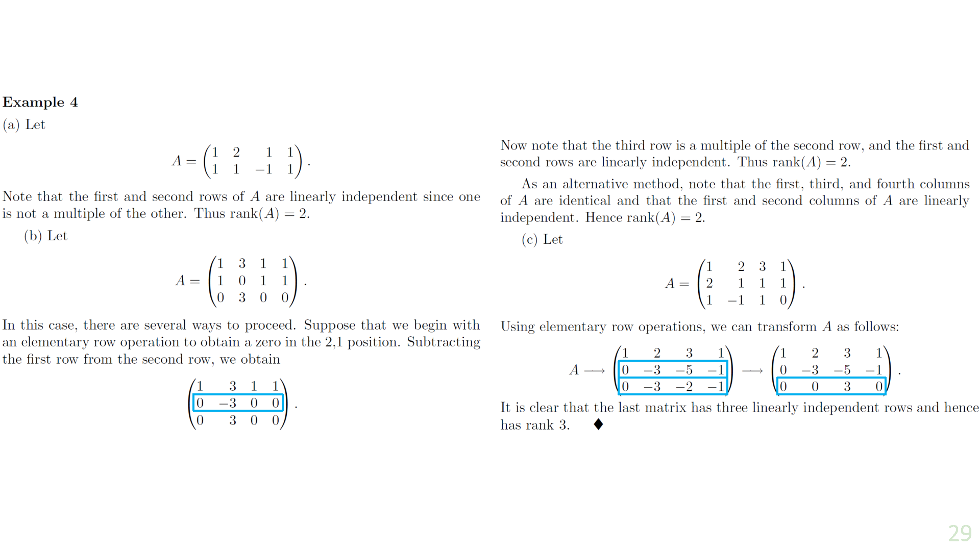
Example 3.2.1 (Rank Determination)

Let

$$A=\left[\begin{array}{ccc}1& 0& 1\\ 0& 1& 1\\ 1& 0& 1\end{array}\right].$$

Observe that the first and second columns of $A$ are linearly independent and that the third column is a linear combination of the first two. Thus,

$$\mathrm{rank}(A)=\dim \mathrm{span}\{\left[\begin{array}{c}1\\ 0\\ 1\end{array}\right],\left[\begin{array}{c}0\\ 1\\ 0\end{array}\right],\left[\begin{array}{c}1\\ 1\\ 1\end{array}\right]\}=2.$$

Example 3.2.2

Let

$$A=\left[\begin{array}{ccc}1& 2& 1\\ 1& 0& 3\\ 1& 1& 2\end{array}\right].$$

If we substract the 1st row of $A$ from rows 2 and 3 (type 3 elementary row operations), the result is

$$\left[\begin{array}{ccc}1& 2& 1\\ 0& -2& 2\\ 0& -1& 1\end{array}\right].$$

If we now substract twice the 1st column from the 2nd and substract the 1st column from the 3rd (type 3 elementary column operations), we obtain

$$\left[\begin{array}{ccc}1& 0& 0\\ 0& -2& 2\\ 0& -1& 1\end{array}\right].$$

It's now obvious that the maximum number of linearly independent columns of this matrix is $2$. Hence the rank of $A$ is $2$.

Theorem 3.6

Let $A$ be an $m\times n$ matrix of rank $r$. Then $r\le m$, $r\le n$, and by means of a finite number of elementary row and column operations, $A$ can be transformed into the matrix

$$D=\left[\begin{array}{cc}{I}_r& {\mathbf{0}}_1\\ {\mathbf{0}}_2& {\mathbf{0}}_3\end{array}\right],$$

where $I_r$ is the $r\times r$ identity matrix and the other blocks are zero matrices. Thus $D_{ii}=1$ for $i\le r$ and $D_{ij}=0$ otherwise.

Example 3.2.3

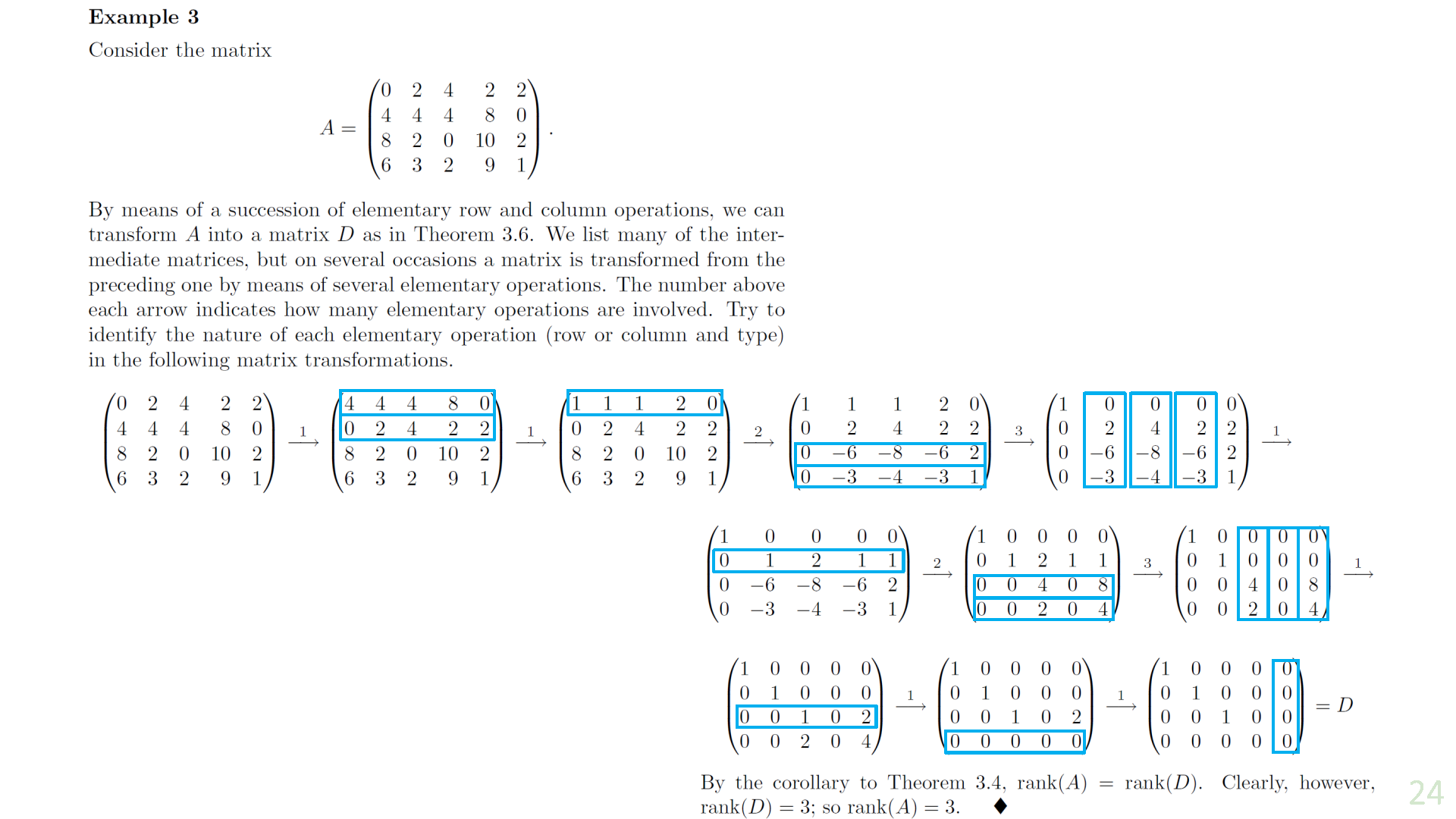
Conclusion about rank

Corollary 1

Let $A$ be an $m\times n$ matrix of rank $r$. Then there exist invertible matrices $B$ (size $m\times m$) and $C$ (size $n\times n$) such that $D=BAC$, where

$$D=\left[\begin{array}{cc}{I}_r& {\mathbf{0}}_1\\ {\mathbf{0}}_2& {\mathbf{0}}_3\end{array}\right]$$

is the $m\times n$ matrix in which ${\mathbf{0}}_1,{\mathbf{0}}_2,{\mathbf{0}}_3$ are zero matrices.

Corollary 2

Let $A$ be an $m\times n$ matrix. Then

• $\mathrm{rank}(A^{\mathrm{\top }})=\mathrm{rank}(A)$.
• The rank of any matrix equals the maximum number of its linearly independent rows; that is, the rank of a matrix is the dimension of the subspace generated by its rows.
• The rows and columns of any matrix generate subspaces of the same dimension, numerically equal to the rank of the matrix.

Corollary 3

Every invertible matrix is a product of elementary matrices

Theorem 3.7

Let $\mathsf{T}:\mathsf{V}\to \mathsf{W}$ and $\mathsf{U}:\mathsf{W}\to \mathsf{Z}$ be linear transformations on finite- dimensional vector spaces $\mathsf{V}\mathsf{,}\mathsf{W}\mathsf{,}\mathsf{Z}$, and let $A$ and $B$ be matrices s.t. the product $AB$ is defined. Then

• $\mathrm{rank}(\mathsf{UT})\le \mathrm{rank}(\mathsf{U})$
• $\mathrm{rank}(\mathsf{UT})\le \mathrm{rank}(\mathsf{T})$
• $\mathrm{rank}(AB)\le \mathrm{rank}(A)$
• $\mathrm{rank}(AB)\le \mathrm{rank}(B)$

Example 3.2.4

The Inverse of a Matrix

Definition: augented matrix

Let $A$ and $B$ be $m\times n$ and $m\times p$ matrices, respectively. By the augmented matrix $(A|B)$, we mean the $m\times (n+p)$ matrix $(AB)$, that is, the matrix whose first $n$ columns are the columns of $A$, and whose last $p$ columns are the columns of $B$.

Let $A$ be an invertible $n\times n$ matrix, and consider the $n\times 2n$ augmented matrix $C=(A|I_n)$. By Exercise 15, we have $A^{-1}C=(A^{-1}A|A^{-1}{I}_n)=(I_n|A^{-1}).(1)$

By Corollary 3 to Theorem 3.6, $A^{-1}$ is the product of elementary matrices, say $A^{-1}=E_p{E}_{p-1}\cdots E_1$. Thus (1) becomes $E_p{E}_{p-1}\cdots E_1(A|I_n)=A^{-1}C=(I_n|A^{-1}).$

Because multiplying a matrix on the left by an elementary matrix transforms the matrix by an elementary row operation (Theorem 3.1 p. 149), we have the following result: If $A$ is an invertible $n\times n$ matrix, then it is possible to transform the matrix $(A|I_n)$ into the matrix $(I_n|A^{-1})$ by means of a finite number of elementary row operations.

Conversely, suppose that $A$ is invertible and that, for some $n\times n$ matrix $B$, the matrix $(A|I_n)$ can be transformed into the matrix $(I_n|B)$ by a finite number of elementary row operations. Let $E_1,E_2,...,E_p$ be the elementary matrices associated with these elementary row operations as in Theorem 3.1; then

$$\begin{array}{}\text{(2)}& E_p{E}_{p-1}\cdots E_1(A|I_n)=(I_n|B).\end{array}$$

Letting $M=E_p{E}_{p-1}\cdots E_1$, we have from (2) that $(MA|M{I}_n)=(I_n|B).$ Hence $MA=I_n$ and $M=B$. It follows that $M=A^{-1}$. So $B=A^{-1}$. Thus we have the following result: If $A$ is an invertible $n\times n$ matrix, and the matrix $(A|I_n)$ is transformed into a matrix of the form $(I_{n}B)$ by means of a finite number of elementary row operations, then $B=A^{-1}$.

If, on the other hand, $A$ is an $n\times n$ matrix that is not invertible, then $\mathrm{rank}(A)<n$. Hence any attempt to transform $(A|I_n)$ into a matrix of the form $(I_n|B)$ by means of elementary row operations must fail because otherwise $A$ can be transformed into $I_n$ using the same row operations. This is impossible, however, because elementary row operations preserve rank. In fact, $A$ can be transformed into a matrix with a row containing only zero entries, yielding the following result: If $A$ is an $n\times n$ matrix that is not invertible, then any attempt to transform $(A|I_n)$ into a matrix of the form $(I_n|B)$ produces a row whose first $n$ entries are zeros.

Example 3.2.5

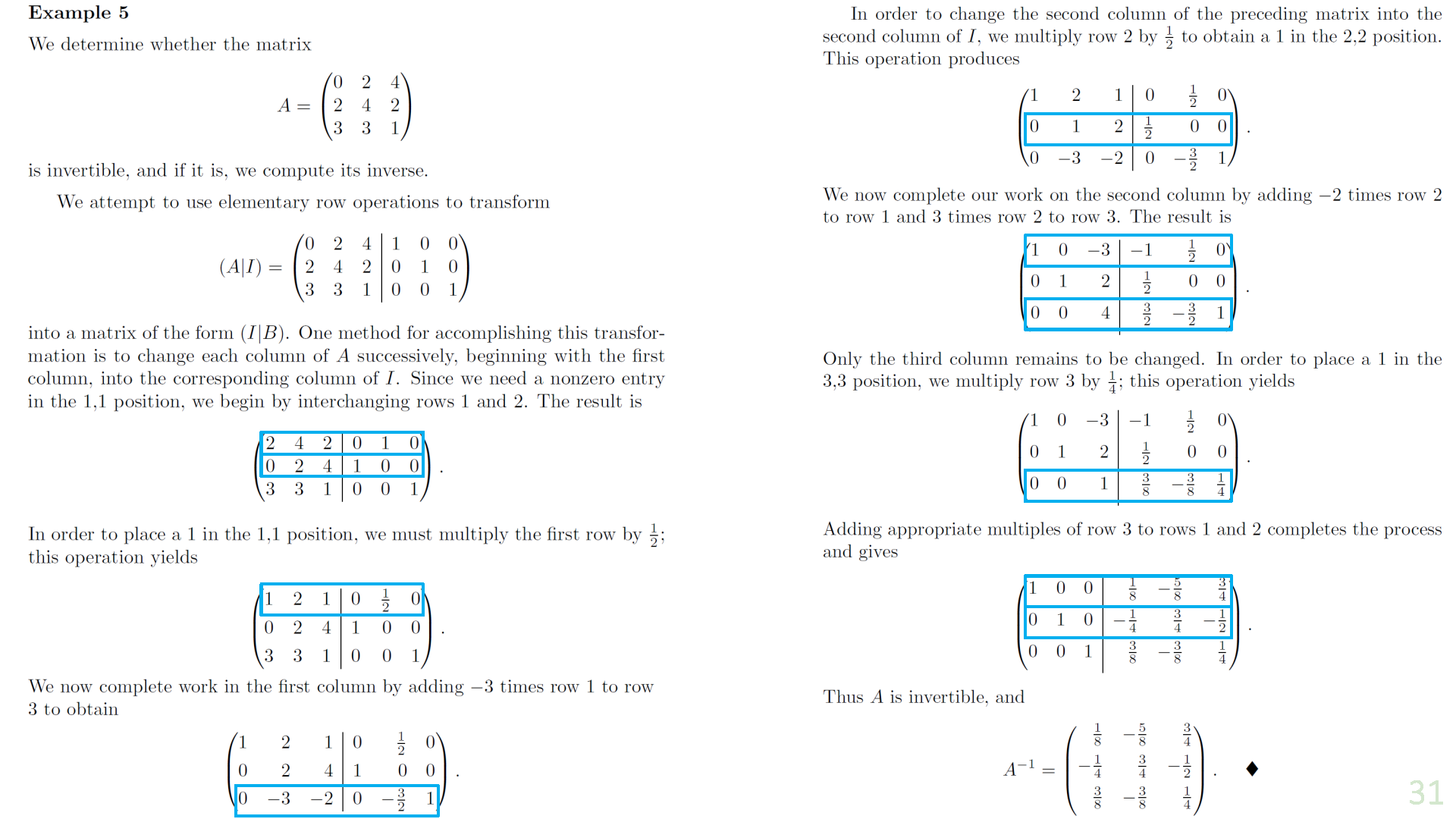
Example 3.2.6

We determine whether the matrix

$$A=\left(\begin{array}{ccc}1& 2& 1\\ 2& 1& -1\\ 1& 5& 4\end{array}\right)$$

is invertible, and if it is, we compute its inverse. Using a strategy similar to the one used in Example 3.2.5, we attempt to use elementary row operations to transform

$$(A|I)=\left[\begin{array}{cccccc}1& 2& 1& 1& 0& 0\\ 2& 1& -1& 0& 1& 0\\ 1& 5& 4& 0& 0& 1\end{array}\right]$$

into a matrix of the form $(I|B)$. We first add $-2$ times row $1$ to row $2$ and $-1$ times row $1$ to row $3$. We then add row $2$ to row $3$. The result,

$$\begin{array}{rl}& \left[\begin{array}{cccccc}1& 2& 1& 1& 0& 0\\ 2& 1& -1& 0& 1& 0\\ 1& 5& 4& 0& 0& 1\end{array}\right]\to \left[\begin{array}{cccccc}1& 2& 1& 1& 0& 0\\ 0& -3& -3& -2& 1& 0\\ 0& 3& 3& -1& 0& 1\end{array}\right]\\ \to & \left[\begin{array}{cccccc}1& 2& 1& 1& 0& 0\\ 0& -3& -3& -2& 1& 0\\ 0& 0& 0& -3& 1& 1\end{array}\right].\end{array}$$

is a matrix with a row whose 1st 3entries are zeros. Therefore $A$ is not invertible.

Example 3.2.7 [core]

Let $\mathsf{T}:{\mathsf{P}}_2(\mathbb{R})\to {\mathsf{P}}_2(\mathbb{R})$ be defined by

$$\mathsf{T}(f(x))=f(x)+f^{\prime }(x)+f^{″}(x),$$

where $f^{\prime }(x)$ and $f^{″}(x)$ denote the first and second derivatives of $f(x)$. We use Corollary 1 of Theorem 2.18 to test $\mathsf{T}$ for invertibility and compute the inverse if $\mathsf{T}$ is invertible. Taking $\beta$ to be the standard ordered basis of ${\mathsf{P}}_2(\mathbb{R})$, we have

$$[\mathsf{T}{]}_{\beta }=\left[\begin{array}{ccc}1& 1& 2\\ 0& 1& 2\\ 0& 0& 1\end{array}\right].$$

Using the method of Examples 5 and 6, $[\mathsf{T}{]}_{\beta }$ is invertible with inverse

$$([\mathsf{T}{]}_{\beta }{)}^{-1}=\left(\begin{array}{ccc}1& -1& 0\\ 0& 1& -2\\ 0& 0& 1\end{array}\right).$$

Thus $\mathsf{T}$ is invertible, and $([\mathsf{T}{]}_{\beta }{)}^{-1}=[{\mathsf{T}}^{-1}{]}_{\beta }$. Hence by Theorem 2.14 (p. 91), we have

$$[{\mathsf{T}}^{-1}(a_0+a_{1}x+a_2{x}^2){]}_{\beta }=\left[\begin{array}{ccc}1& -1& 0\\ 0& 1& -2\\ 0& 0& 1\end{array}\right]\left[\begin{array}{c}{a}_0\\ a_1\\ a_2\end{array}\right]=\left[\begin{array}{c}{a}_0-a_1\\ a_1-2a_2\\ a_2\end{array}\right]$$

Therefore

$${\mathsf{T}}^{-1}(a_0+a_{1}x+a_2{x}^2)=(a_0-a_1)+(a_1-2a_2)x+a_2{x}^2.$$

3.3 Systems of Linear Equations - Theoretical Aspects

The system of equations

$$\{\begin{array}{l}{a}_{11}{X}_1+a_{12}{X}_2+\cdots +a_{1n}{X}_n=b_1\\ a_{21}{X}_1+a_{22}{X}_2+\cdots +a_{2n}{X}_n=b_2\\ ⋮\\ a_{m1}{X}_1+a_{m2}{X}_2+\cdots +a_{mn}{X}_n=b_m\end{array}$$

where $a_{ij}$ and $b_i$ are scalars in a field $F$ and $x_1,x_2,\cdots ,x_n$ are $n$ variables taking values in $F$, is called a system of $m$ linear equations in $n$ unknowns over the field $F$.

The $m\times n$ matrix

$$A=\left[\begin{array}{cccc}{a}_{11}& a_{12}& \cdots & a_{1n}\\ a_{21}& a_{22}& \cdots & a_{2n}\\ ⋮& ⋮& & ⋮\\ a_{m1}& a_{m2}& \cdots & a_{mn}\end{array}\right]$$

is called the coefficient matrix of the system $(S)$.

We can write the system as a single matrix equation

$$Ax=b,$$

where

$$x=\left(\begin{array}{c}{x}_1\\ x_2\\ ⋮\\ x_n\end{array}\right),b=\left(\begin{array}{c}{b}_1\\ b_2\\ ⋮\\ b_m\end{array}\right).$$

To exploit the results that we have developed, we often consider a system of linear equations as a single matrix equation.

A solution to the system $(S)$ is an $n$-tuple

$$s=(s_1,s_2,\dots ,s_n{)}^{\mathrm{\top }}\in {\mathsf{F}}^n$$

such that $As=b$. The set of all solutions to the system $(S)$ is called the solution set of the system. System $(S)$ is consistent if its solution set is nonempty; otherwise it is inconsistent.

Example 3.3.1

(a) Consider the system

$$\{\begin{array}{l}{x}_1+x_2=3\\ x_1-x_2=1\end{array}$$

The solution is unique: $x_1=2$, $x_2=1$.

In matrix form:

$$\left(\begin{array}{cc}1& 1\\ 1& -1\end{array}\right)\left(\begin{array}{c}{x}_1\\ x_2\end{array}\right)=\left(\begin{array}{c}3\\ 1\end{array}\right).$$

(b) Consider the system

$$\{\begin{array}{l}2x_1+3x_2+x_3=1\\ x_1-x_2+2x_3=6\end{array}$$

which has infinitely many solutions, such as: $s=(-6,2,7{)}^{\mathrm{\top }}$ and $s=(8,-4,-3{)}^{\mathrm{\top }}$.

(c) Consider

$$\{\begin{array}{l}{x}_1+x_2=0\\ x_1+x_2=1\end{array}$$

that is

$$\left[\begin{array}{cc}1& 1\\ 1& 1\end{array}\right]\left[\begin{array}{c}{x}_1\\ x_2\end{array}\right]=\left[\begin{array}{c}0\\ 1\end{array}\right]$$

It's evident that this system has no solutions. Thus we see that a system of linear equations can have one, many, or no solutions.

homogeneous

Definitions: homogeneous

A system $Ax=b$ is said to be homogeneous if $b=0$, otherwise nonhomogeneous.

Theorem 3.8

Let $Ax=0$ be a homogeneous system of $m$ linear equations in $n$ unknowns over a field $F$. Let $\mathsf{K}$ denote the set of all solutions to $Ax=0$. Then $\mathsf{K}=\mathsf{N}({\mathsf{L}}_A)$; hence $\mathsf{K}$ is a subspace of ${\mathsf{F}}^n$ of dimension $n-\mathrm{rank}({\mathsf{L}}_A)=n-\mathrm{rank}(A)$.

Corollary

If $m<n$, the system $Ax=0$ has a nonzero solution.

Example 3.3.2 [core]

(a) Consider the system

$$\{\begin{array}{l}{x}_1+2x_2+x_3=0\\ x_1-x_2+x_3=0\end{array}$$

Let

$$A=\left(\begin{array}{ccc}2& 1& 1\\ 0& 0& 1\\ -1& -1& 1\end{array}\right)$$

be the coefficient matrix of this system. It is clear that $\mathrm{rank}(A)=2.$ If $K$ is the solution set of this system, then $\dim (K)=3-2=1.$ Thus any nonzero solution constitutes a basis for $K.$ For example, since

$$\left(\begin{array}{c}1\\ -2\\ 3\end{array}\right)$$

is a solution to the given system, it is a basis for $K.$ Thus any vector in $K$ is of the form

$$\left(\begin{array}{c}t\\ -2t\\ 3t\end{array}\right)$$

where $t\in \mathbb{R}.$

(b) Consider the system $x_1-2x_2+x_3=0$ of one equation in three unknowns. If $A=\left(\begin{array}{ccc}1& -2& 1\end{array}\right)$ is the coefficient matrix, then $\mathrm{rank}(A)=1.$ Hence if $K$ is the solution set, then $\dim (K)=3-1=2.$ Note that

$$\left[\begin{array}{c}2\\ 1\\ 0\end{array}\right]\text{ and }\left[\begin{array}{c}-1\\ 0\\ 1\end{array}\right]$$

are linearly independent vectors in $\mathsf{K}$. Thus they constitute a basis for $\mathsf{K}$, so that

$$\mathsf{K}=\{t_1\left[\begin{array}{c}2\\ 1\\ 0\end{array}\right]+t_2\left[\begin{array}{c}-1\\ 0\\ 1\end{array}\right]:t_1,t_2\in \mathbb{R}\}.$$

Theorem 3.9

Let $K$ be the solution set of a system $Ax=b$, and let ${\mathsf{K}}_H$ be the solution set of the corresponding homogeneous system $Ax=0$. Then for any solution $s$ to $Ax=b$,

$$K=\{s\}+{\mathsf{K}}_H=\{s+k:k\in {\mathsf{K}}_H\}.$$

Example 3.3.3

(a) Consider the system

$$\{\begin{array}{l}{x}_1+2x_2+x_3=7\\ x_1+x_2-x_3=-4.\end{array}$$

The corresponding homogeneous system is the system in Example 3.3.2(a). It is easily verified that

$$s=\left(\begin{array}{c}1\\ 1\\ 4\end{array}\right)$$

is a solution to the preceding nonhomogeneous system. So the solution set of the system is

$$\mathsf{K}=\left(\begin{array}{c}1\\ 1\\ 4\end{array}\right)+t\left(\begin{array}{c}1\\ -2\\ 3\end{array}\right),t\in \mathbb{R}$$

by Theorem 3.9.

(b) Consider the system

$$2x_1-2x_2+x_3=4.$$

The corresponding homogeneous system is the system in Example 3.3.2(b). Since

$$s=\left(\begin{array}{c}4\\ 0\\ 0\end{array}\right)$$

is a solution to the given system, the solution set $\mathsf{K}$ can be written as

$$\mathsf{K}=\left(\begin{array}{c}4\\ 0\\ 0\end{array}\right)+t_1\left(\begin{array}{c}2\\ 1\\ 0\end{array}\right)+t_2\left(\begin{array}{c}-1\\ 0\\ 1\end{array}\right):t_1,t_2\in \mathbb{R}.$$

Theorem 3.10

Theorem 3.10

Let $Ax=b$ be a system of $n$ linear equations in $n$ unknowns. If $A$ is invertible, then the system has exactly one solution, namely,

$$x=A^{-1}b.$$

Conversely, if the system has exactly one solution, then $A$ is invertible.

Example 3.3.4

Consider the system:

$$\{\begin{array}{l}2x_2+4x_3=2\\ 2x_1+4x_2+2x_3=3\\ 3x_1+3x_2+x_3=1\end{array}$$

Using the inverse matrix of the coefficient matrix, the unique solution is

$$\left(\begin{array}{c}{x}_1\\ x_2\\ x_3\end{array}\right)=A^{-1}b=\left(\begin{array}{c}-\frac{7}{8}\\ -\frac{5}{4}\\ \frac{1}{8}\end{array}\right).$$

Theorem 3.11

Theorem 3.11

Let $Ax=b$ be a system of linear equations. Then the system is consistent if and only if

$$\mathrm{rank}(A)=\mathrm{rank}(A|b).$$

Example 3.3.5

Recall the system of equations

$$\{\begin{array}{l}{x}_1+x_2=0,\\ x_1+x_2=1.\end{array}$$

in Example 3.3.1(c). Since

$$A=\left(\begin{array}{cc}1& 1\end{array}\right),(A|b)=\left(\begin{array}{ccc}1& 1& 0\\ 1& 1& 1\end{array}\right),$$$$\mathrm{rank}(A)=1,\mathrm{rank}(A|b)=2.$$

Because the two ranks are unequal, the system has no solutions.

Example 3.3.6

We can use Theorem 3.11 to determine whether $(3,3,2)$ is in the range of the linear transformation $\mathsf{T}:{\mathbb{R}}^3\to {\mathbb{R}}^3$ defined by

$$\mathsf{T}(a_1,a_2,a_3)=(a_1+a_2+a_3,a_1{a}_2+a_3,a_1+a_3).$$

We check if $(3,3,2)\in \mathsf{R}\mathsf{(}\mathsf{T}\mathsf{)}$ by solving the system

$$\begin{array}{rlrl}& x_1+x_2& & +x_3=3,\\ & x_1-x_2& & +x_3=3,\\ & x_1& & +x_3=2\end{array}$$

Since the rank of the coefficient matrix is 2 but the augmented matrix is 3, this system has no solutions. Hence $(3,3,2)\notin \mathsf{R}\mathsf{(}\mathsf{T}\mathsf{)}.$

3.4 Systems of Linear Equations - Computational Aspects

Definition: equivalent

Two systems of linear equations are called equivalent if they have the same solution set.

Theorem 3.13

Let $Ax=b$ be a system of $m$ linear equations in $n$ unknowns, and let $C$ be an invertible $m\times m$ matrix. Then $(CA)x=Cb$ is equivalent to $Ax=b$.

Corollary

If $(A^{\prime }|b^{\prime })$ is obtained from $(A|b)$ by a finite number of elementary row operations, then the system $A^{\prime }x=b^{\prime }$ is equivalent to the original system.

Gaussian Elimination Method Outline:

1. Form the augmented matrix $(A|b)$.
2. Use elementary row operations to transform $(A|b)$ into reduced row echelon form.
3. Solve the system from the reduced form using back substitution.

We now describe a method for solving any system of linear equations.

Consider the system:

$$\begin{array}{rlrlrlrlrl}3& x_1+2& & x_2+3& & x_3-2& & x_4& & =1,\\ & x_1+& & x_2+& & x_3& & & & =3,\\ & x_1+2& & x_2+& & x_3-& & x_4& & =2.\end{array}$$

First, form the augmented matrix:

$$\left(\begin{array}{ccccc}3& 2& 3& -2& 1\\ 1& 1& 1& 0& 3\\ 1& 2& 1& -1& 2\end{array}\right).$$

Then perform elementary row operations to transform it into an upper triangular matrix in reduced row echelon form using steps involving row interchanges, scaling, and elimination as described.

1. In the leftmost nonzero column, create a 1 in the first column;

$$\left(\begin{array}{ccccc}1& 2& 1& -1& 2\\ 1& 1& 1& 0& 3\\ 3& 2& 3& -2& 1\end{array}\right).$$

2. By means of type 3 row operations, use the first row to obtain zeros in the remaining positions of the leftmost nonzero column;$$\left(\begin{array}{ccccc}1& 2& 1& -1& 2\\ 0& -1& 0& 1& 1\\ 0& -4& 0& 1& -5\end{array}\right).$$
3. Create a 1 in the next row in the leftmost possible column, without using previous rows;

$$\left(\begin{array}{ccccc}1& 2& 1& -1& 2\\ 0& 1& 0& -1& -1\\ 0& -4& 0& 1& -5\end{array}\right).$$

4. Use type 3 elementary row operations to obtain zeros below the 1 created in the preceding step;

$$\left(\begin{array}{ccccc}1& 2& 1& -1& 2\\ 0& 1& 0& -1& -1\\ 0& 0& 0& -3& -9\end{array}\right).$$

5. Repeat 3 and 4 until no nonzero rows remain;

$$\left(\begin{array}{ccccc}1& 2& 1& -1& 2\\ 0& 1& 0& -1& -1\\ 0& 0& 0& 1& 3\end{array}\right).$$

6. Work upward, beginning with the last nonzero row, and add multiples of each row to the rows above. Repeat the process for each preceding row until it is performed with the 2nd row, at which time the reduction process is completed.

$$\left(\begin{array}{ccccc}1& 0& 1& 0& 1\\ 0& 1& 0& 0& 2\\ 0& 0& 0& 1& 3\end{array}\right).$$

Definition: Reduced row echelon form

A matrix is said to be in reduced row echelon form if it satisfies: (a) Any row containing a nonzero entry precedes any row with all zero entries.

(b) The first nonzero entry in each row is the only nonzero entry in its column.

(c) The first nonzero entry in each row is 1 and it occurs to the right of the first nonzero entry in the preceding row.

The method described with forward elimination and back substitution is known as Gaussian elimination.

Theorem 3.14

Gaussian elimination transforms any matrix into its reduced row echelon form.

Theorem 3.15

Let $Ax=b$ be a system of $r$ nonzero equations in $n$ unknowns with $\mathrm{rank}(A)=\mathrm{rank}(A|b)=r.$ Suppose $(A|b)$ is in reduced row echelon form. Then:

• $\mathrm{rank}(A)=r$.
• If the general solution is

$$s=s_0+t_1{u}_1+\cdots +t_{n-r}{u}_{n-r},$$

then $\{u_1,\dots ,u_{n-r}\}$ is a basis for the solution set of the corresponding homogeneous system, and $s_0$ is the solution to the original system.

Theorem 3.16

Let $A$ be an $m\times n$ matrix of rank $r>0,$ and $B$ the reduced row echelon form of $A.$ Then:

(a) The number of nonzero rows in $B$ is $r.$

(b) For each $i=1,\dots ,r,$ there is a column $b_{j_i}$ of $B$ such that $b_{j_i}=e_i.$

(c) The columns of $A$ numbered $j_1,\dots ,j_r$ are linearly independent.

(d) For each $k=1,\dots ,n,$ if column $k$ of $B$ is a linear combination $\sum d_i{e}_i,$ then column $k$ of $A$ is $\sum d_i{a}_{j_i}$.

Corollary

The reduced row echelon form of a matrix is unique.

Example 3.4.2

Let

$$A=\left(\begin{array}{lllll}2& 4& 6& 2& 4\\ 1& 2& 3& 1& 1\\ 2& 4& 8& 0& 0\\ 3& 6& 7& 5& 9\end{array}\right).$$

The reduced row echelon form of $A$ is

$$B=\left(\begin{array}{ccccc}1& 2& 0& 4& 0\\ 0& 0& 1& -1& 0\\ 0& 0& 0& 0& 1\\ 0& 0& 0& 0& 0\end{array}\right).$$

Since $B$ has three nonzero rows, the rank of $A$ is 3 . The first, third, and fifth columns of $B$ are $e_1,e_2$, and $e_3$; so Theorem 3.16(c) asserts that the first, third, and fifth columns of $A$ are linearly independent.

Let the columns of $A$ be denoted $a_1,a_2,a_3,a_4$, and $a_5$. Because the second column of $B$ is $2e_1$, it follows from Theorem 3.16(d) that $a_2=2a_1$, as is easily checked. Moreover, since the fourth column of $B$ is $4e_1+(-1)e_2$, the same result shows that

$$a_4=4a_1+(-1)a_3.$$

Example 3.4.3

The set

$$S=\{2+x+2x^2+3x^3,4+2x+4x^2+6x^3,6+3x+8x^2+7x^3,2+x+5x^3,4+x+9x^3\}$$

generates a subspace $\mathsf{V}$ of ${\mathsf{P}}_3(\mathbb{R})$. To find a subset of $S$ that is a basis for $\mathsf{V}$, we consider the subset

$$S^{\prime }=\{(2,1,2,3),(4,2,4,6),(6,3,8,7),(2,1,0,5),(4,1,0,9)\}$$

consisting of the images of the polynomials in $S$ under the standard representation of ${\mathsf{P}}_3(\mathbb{R})$ with respect to the standard ordered basis. Note that the $4\times 5$ matrix in which the columns are the vectors in $S^{\prime }$ is the matrix $A$ in Example 2. From the reduced row echelon form of $A$, which is the matrix $B$ in Example 2, we see that the first, third, and fifth columns of $A$ are linearly independent and the second and fourth columns of $A$ are linear combinations of the first, third, and fifth columns. Hence

$$\{(2,1,2,3),(6,3,8,7),(4,1,0,9)\}$$

is a basis for the subspace of ${\mathbb{R}}^4$ that is generated by $S^{\prime }$. It follows that

$$\{2+x+2x^2+3x^3,6+3x+8x^2+7x^3,4+x+9x^3\}$$

is a basis for the subspace $\mathsf{V}$ of ${\mathsf{P}}_3(\mathbb{R})$.

Example 3.4.4 [mid-term]

Let

$$V=\{(x_1,x_2,x_3,x_4,x_5)\in {\mathbb{R}}^5:x_1+7x_2+5x_3-4x_4+2x_5=0\}.$$

It is easily verified that $\mathsf{V}$ is a subspace of ${\mathbb{R}}^5$ and that

$$S=\{(-2,0,0,-1,-1),(1,1,-2,-1,-1),(-5,1,0,1,1)\}$$

is a linearly independent subset of $\mathsf{V}$.

To extend $S$ to a basis for $\mathsf{V}$, we first obtain a basis $\beta$ for $\mathsf{V}$. To do so, we solve the system of linear equations that defines $\mathsf{V}$. Since in this case $\mathsf{V}$ is defined by a single equation, we need only write the equation as

$$x_1=-7x_2-5x_3+4x_4-2x_5$$

and assign parametric values to $x_2,x_3,x_4,x_5$. If $x_2=t_1,x_3=t_2,x_4=t_3$, and $x_5=t_4$, then the vectors in $\mathsf{V}$ have the form

$$\begin{array}{rl}(x_1,x_2,x_3,x_4,x_5)=& (-7t_1-5t_2+4t_3-2t_4,t_1,t_2,t_3,t_4)\\ =& t_1(-7,1,0,0,0)+t_2(-5,0,1,0,0)\\ & +t_3(4,0,0,1,0)+t_4(-2,0,0,0,1).\end{array}$$

Hence

$$\beta =\{(-7,1,0,0,0),(-5,0,1,0,0),(4,0,0,1,0),(-2,0,0,0,1)\}$$

is a basis for $\mathsf{V}$ by Theorem 3.15.

The matrix whose columns consist of the vectors in $S$ followed by those $\beta$ is

$$\left(\begin{array}{ccccccc}-2& 1& -5& -7& -5& 4& -2\\ 0& 1& 1& 1& 0& 0& 0\\ 0& -2& 0& 0& 1& 0& 0\\ -1& -1& 1& 0& 0& 1& 0\\ -1& -1& 1& 0& 0& 0& 1\end{array}\right)$$

and its reduced row echelon form is

$$\left(\begin{array}{ccccccc}1& 0& 0& 1& 1& 0& -1\\ 0& 1& 0& 0& -.5& 0& 0\\ 0& 0& 1& 1& .5& 0& 0\\ 0& 0& 0& 0& 0& 1& -1\\ 0& 0& 0& 0& 0& 0& 0\end{array}\right).$$

Thus

$$\{(-2,0,0,-1,-1),(1,1,-2,-1,-1),(-5,1,0,1,1),(4,0,0,1,0)\}$$

is a basis for $\mathsf{V}$ containing $S$.