Sensor Integration and Signal processing Part II

Average filter

Average is sum of a given data set divided by the number of data in it.

For example,If the given data set contains $k$ datum $(x_1,x_2,\cdots ,x_4)$ the average is obtained by the following expression:

$${\overline{x}}_k=\frac{x_1+x_2+\cdots +x_k}{k}.$$

The expression above treats whole data in a single batch and thus called 'batch expression'.

The recursive expression boosts computational efficiency by reusing prior results (notably for large datasets) and cuts memory usage, needing only the previous average, new data, and total data count, unlike Average Filter which requires the full dataset.

For the averaging filter, we can get the following recursive expression.

$${\overline{x}}_k=\frac{k-1}{k}{\overline{x}}_{k-1}+\frac{1}{k}{x}_k$$

If we use the Equation above to get average, only the average computed in previous step(${\overline{x}}_{k-1}$), total number of datum in the data set($k$), and freshly added datum(${\overline{x}}_k$) are all we need. Here, we do not need whole datum in the data set. This is why a recursive expression is useful for computing average of a data set with a datum being added sequentially.

This equation could be simplified even further. If we define $\alpha \equiv k/(k-1)$,following relationship between $\alpha$ and $k$ stands:

$$\alpha \equiv \frac{k-1}{k}=1-\frac{1}{k},\frac{1}{k}=1-\alpha .$$

And we can get a simplified form of the recursive expression:

$$\begin{array}{rl}{\overline{x}}_k& =\frac{k-1}{k}{\overline{x}}_{k-1}+\frac{1}{k}{x}_k\\ & =\alpha {\overline{x}}_{k-1}+(1-\alpha )x_k.\end{array}$$

The name of this Equation is 'average filter'.

The average filter is applicable to both average calculation and sensor initialization, as perfectly exemplified by a digital weight scale.

• The zero point of a digital weight scale changes continuously for various reasons, so an initialization process is required to determine the zero point by collecting measurements over a certain period after power-on. If all measurements have to be stored to calculate the average, an expensive microprocessor will be needed, which is obviously an unfavorable option. This can be avoided by adopting an average filter.

Figure 1: Average filter.

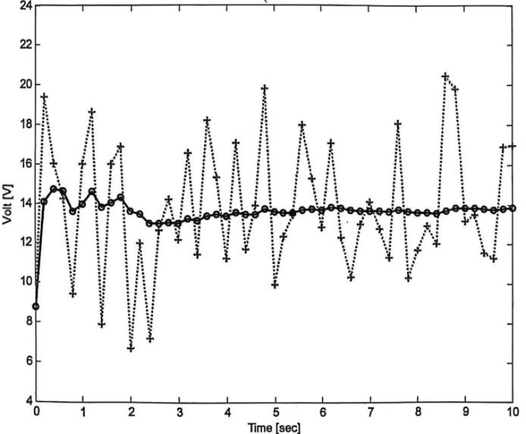
The plot of the average filter's voltage results shows violent fluctuations in raw measurements versus a stable filtered output. As data accumulates, noise fades and the output approaches the true voltage average; this noise-filtering property of averaging is why it is named a "filter".

Moving average filter

5-day moving average curve plots the moving average of stock prices over a 5-day window, which is used to track the medium-to-long-term trends of stock prices and eliminate confusion caused by daily fluctuations. This chapter will elaborate on the concept of the moving average.

Moving average is an average of not all the data in the data set, but of certain number of recent measurements. This method discards the oldest data whenever a new datum comes in and in that way it maintains the number of datum to get the average.

Moving average of $n$ datum is expressed as following:

$${\overline{x}}_k=\frac{x_{k-n+1}+x_{k-n+2}+\cdots +x_k}{n}.$$

Beware that ${\overline{x}}_k$ used here for moving average filter has different meaning from that used to describe average filter. In the average filter, ${\overline{x}}_k$ meant the average of $k$ datum. In contrast, ${\overline{x}}_k$ for moving average filter is the average of $n$ datum from $(k-n+1{)}^{\text{th}}$ to $k^{\text{th}}$ datum but not the average of all $k$ datum.

Leaving ${\overline{x}}_k$ on the left hand side we get recursive expression:

$${\overline{x}}_k={\overline{x}}_{k-1}+\frac{x_k-x_{k-n}}{n}$$

This is 'moving average filter'. It is not as neat as average filter but still is in recursive expression.

Load required for computation of an average is not increased even after a new datum is fed in. This inherent characteristic of low computing load gives little room for recursive expression to provide any advantage unlike average filter.

The moving average filter involves a direct trade-off between noise reduction and phase lag. While increasing the sample size ($n$) enhances noise suppression, it introduces delays that prevent the output from reflecting real-time variations. Conversely, reducing $n$ improves responsiveness but sacrifices filtering performance.

In practice, the value of $n$ must be tailored to the signal's dynamics:

• For rapid variations: Use a smaller $n$ to minimize lag and ensure quick tracking.
• For slow variations: Use a larger $n$ to maximize noise reduction and achieve a stable average.

The Moving Average Filter involves a fundamental trade-off between noise suppression and response time:

• Higher $n$: Enhances noise reduction but introduces latency, hindering real-time tracking.
• Lower $n$: Enables faster response to data changes but sacrifices filtering quality.

Conclusion: The optimal value for $n$ must be chosen based on the signal's characteristics. Furthermore, unlike the standard average filter, its recursive implementation offers limited algorithmic advantages.

1st order Low-pass filter

When moving average filter is brought into real world, you will notice that reducing noise and tracking variation of the given data at the same time is not an easy task. Quite frequently, even if you change the number of datum to get average, the result is not so satisfactory.

Breaking the definition of moving average in Equation into each term.

$${\overline{x}}_k=\frac{x_{k-n+1}+x_{k-n+2}+\cdots +x_k}{n}=\frac{1}{n}{x}_{k-n+1}+\frac{1}{n}{x}_{k-n+2}+\cdots +\frac{1}{n}{x}_k$$

From this expression, we see that each term in the moving average has same weighting ($1/n$) to the other. Most recent datum ($x_k$) and the oldest datum ($x_{k-n+1}$) have same weight in the average.

An aircraft has an attitude sensor which returns 50 measurements in 1 second. Moving average filter of the flight management computer computes an average with 50 collected datum($n=50$). In this case, the oldest datum used to compute the average is the one measured 1 second ago. When the aircraft is in flight, which one, between the one measured 1 second ago and the one measured most recent, would be closer to current attitude?

The answer would most possibly be the one measured most recent. However, moving average filter processes all measurements with equal weighting.

Unlike we have done so far, recursive expression will be directly given for low-pass filter. The accurate name for this filter is '1st order low-pass filter'.

$${\overline{x}}_k=\alpha {\overline{x}}_{k-1}+(1-\alpha )x_k.$$

Where $\alpha$ is a constant in the range of $0<\alpha <1$.

From now on, we will use the term 'estimate' instead of 'average' or 'mean' because ${\overline{x}}_k$ in a low-pass filter has nothing to do with average. According to the Equation, previous estimate ${\overline{x}}_{k-1}$ is computed as following:

$${\overline{x}}_{k-1}=\alpha {\overline{x}}_{k-2}+(1-\alpha )x_{k-1}.$$

Thus:

$$\begin{array}{rl}{\overline{x}}_k& =\alpha {\overline{x}}_{k-1}+(1-\alpha )x_k\\ & =\alpha [\alpha {\overline{x}}_{k-2}+(1-\alpha )x_{k-1}]+(1-\alpha )x_k\\ & ={\alpha }^2{\overline{x}}_{k-2}+\alpha (1-\alpha )x_{k-1}+(1-\alpha )x_k\\ & ={\alpha }^2[\alpha {\overline{x}}_{k-3}+(1-\alpha )x_{k-2}]+\alpha (1-\alpha )x_{k-1}+(1-\alpha )x_k\\ & ={\alpha }^3{\overline{x}}_{k-3}+{\alpha }^2(1-\alpha )x_{k-2}+\alpha (1-\alpha )x_{k-1}+(1-\alpha )x_k\end{array}$$

Therefore, there are following relationships among measurements:

$$\cdots <{\alpha }^2(1-\alpha )<\alpha (1-\alpha )<1-\alpha .$$

Equation confirms that weighting coefficients decrease as data ages. Consequently, older data points exert less influence on the final estimate, ensuring the filter prioritizes recent information.

The estimate of a 1st-order low-pass filter is highly sensitive to the coefficient $\alpha$:

• Small $\alpha$ (e.g., $0.4$): Higher noise levels but faster response with minimal lag.
• Large $\alpha$ (e.g., $0.9$): Superior noise reduction at the cost of significant time delay.

1st order low-pass-filter is also known as 'exponentially weighted moving average filter'.

Kalman filter algorithm

It receives only one input (measurement, $z_k$) and returns one output (estimate, ${\hat{x}}_k$).

Internal process is done through a four-step computation.

1. Step I (Prediction): Computes predicted variables (denoted by a - superscript) based on the system model.
2. Step II (Kalman Gain): Calculates the Kalman gain using the output from Step I and external presets/noise characteristics (H and R).
3. Step III (Estimation): Computes the current estimate using the measurement input and Step I's prediction (conceptually similar to a low-pass filter).
4. Step IV (Error Covariance): Computes the error covariance to evaluate the estimate's accuracy and determine its reliability.

The Kalman filter can be distilled into a continuous recursive loop comprising two main phases: Prediction and Estimation.

• Prediction Process (Step I): Utilizes the previous state and system parameters ($A$ and $Q$) to compute the predicted state (${\hat{x}}_k^{-}$ and $P_k^{-}$).
• Estimation Process (Steps II-IV): Incorporates the current measurement ($z_k$) alongside parameters ($H$ and $R$) to compensate for prediction errors, yielding the final optimal estimate (${\hat{x}}_k,P_k$).

Summary: The algorithm operates as a simple closed loop: Predict state → Compensate with measurement → Repeat.

There was a reason why low-pass filter has been mentioned so frequently whenever Kalman filter was brought up. Let us look at the expression for computing an estimate in Step III for examination.

$${\hat{x}}_k={\hat{x}}_k^{-}+K_k(z_k-H{\hat{x}}_k^{-})$$

where $z_k$ means measurement and ${\hat{x}}_k^{-}$ means prediction.

Simply change:

$$\begin{array}{cc}\begin{array}{rl}{\hat{x}}_k& ={\hat{x}}_k^{-}+K_k(z_k-H{\hat{x}}_k^{-})\\ & ={\hat{x}}_k^{-}+K_k{z}_k-K_{k}H{\hat{x}}_k^{-}\\ & =(I-K_{k}H){\hat{x}}_k^{-}+K_k{z}_k\\ & =(I-K_k){\hat{x}}_k^{-}+K_k{z}_k\text{ If }H=I\end{array}& \begin{array}{rl}{\hat{x}}_k& =\alpha {\overline{x}}_{k-1}+(1-\alpha )x_k\\ & =(1-K){\overline{x}}_{k-1}+(1-(1-K))x_k\\ & =(1-K){\overline{x}}_{k-1}+K{x}_k\end{array}\end{array}$$

Compare this expression with Equation, which is for computation of an estimate in Kalman filter.

Kalman filter is almost the same. The way it assigns weighting is even same with the only difference lying in the fact that Kalman filter is not using the previous estimate but prediction.

For Kalman filter algorithm:

$${\hat{x}}_k={\hat{x}}_k^{-}+K_k(z_k-H{\hat{x}}_k^{-})$$

First of all, a prediction($x$) and a new measurement($z$) are required.

Now the only variable left is Kk. This is called 'Kalman gain' and if the value of this variable is known, the new estimate could be computed.

$$K_k=P_k^{-}{H}^{\mathrm{\top }}(H{P}_k^{-}{H}^{\mathrm{\top }}+R{)}^{-1}$$

We will take a look into an error covariance which is the last step of the estimation process

$$P_k=P_k^{-}-K_{k}H{P}_k^{-}$$

Error covariance indicates the difference between the estimate from Kalman filter and the true but unknown value. In other words, error covariance is a degree of accuracy of the estimate.

If $P_k$ is large, the error of the estimate is large and if $P_k$ is small, the error of the estimate is small.

There is a following relationship between $P_k$ and its estimate(${\hat{x}}_k$)and error covariance($P_k$).

$$x_k\sim \mathcal{N}({\hat{x}}_k,P_k).$$

This basically means the variable $x_k$ follows a normal distribution with mean ${\hat{x}}_k$ , and covariance $P_k$, but there is a lot more deep meaning in here.

That is, Kalman filter computes probability distribution of the estimate of the variable $x_k$ and selects the one with highest probability as the estimate.

This means that if we draw the probability of the values that $x_k$ could have, it comes out as a bellshaped distribution. And the width of this bell-shaped curve is determined by $P_k$.

Error covariance is defined as the following.

$$P_k=\mathbb{E}[(x_k-{\hat{x}}_k)(x_k-{\hat{x}}_k{)}^{\mathrm{\top }}].$$

where $\mathbb{E}[\cdot ]$ is an operator to compute the mean of the variable inside the curly brackets. $x_k-{\hat{x}}_k$ in the right hand side means the difference between the true but unknown and the estimate, i.e.the error of the estimate. In other words, the error covariance is the mean of the square of the error of the estimate. This is why the size of the error covariance is proportional to the error of the estimate.

In the prediction procedure, how the estimate ${\hat{x}}_k$ will vary when time changes from $t_k$ to $t_{k+1}$ is predicted. In other words, it predicts what value will the estimate of current time point have at the next time point $t_{k+1}$.

$$\begin{array}{rl}& {\hat{x}}_{k+1}=A{\hat{x}}_k\\ & P_{k+1}^{-}=A{P}_k{A}^{\mathrm{\top }}+Q\end{array}$$

Here, ${\hat{x}}_k$ and $P_k$ are the values calculated from Steps III and IV, respectively. And $A$ and $Q$ are already defined by the system model. The other variables in the system model such as $H$ and $R$ are not used.

Please pay attention to the notation for the prediction. The subscript ‘$k+1$'attached to indicate that it is the value at the time point t_{k+1}$ and the superscript '-' for indicating that it is a prediction.

Now let us examine the expression to compute the estimate in Kalman filter.

Unlike a 1st-order low-pass filter, the Kalman filter does not directly reuse the previous estimate ( ${\hat{x}}_{k-1}$ ) Instead, it incorporates an intermediate prediction step, leading to specific terminology:

• A Priori Estimate: The prediction (${\hat{x}}_k^{-}$), derived from the previous estimate before the current measurement is considered.

$${\hat{x}}_k^{-}=A{\hat{x}}_{k-1}.$$

• A Posteriori Estimate: The final estimate ( ${\hat{x}}_k$ ), computed after updating the a priori estimate with the new measurement.

$$\begin{array}{rl}{\hat{x}}_k& ={\hat{x}}_k^{-}+K_k(z_k-H{\hat{x}}_k^{-})\\ & =A{\hat{x}}_{k-1}+K_k(z_k-HA{\hat{x}}_{k-1})\end{array}$$

In the expression above, $H{\hat{x}}_k^{-}$ has the meaning of 'the measurement computed with the prediction.' In other words, it is the prediction of the measurement.

The quality of prediction is determined by how close the system model is to the actual system and the performance of estimation is determined by the prediction.

It is not an exaggeration to say that the performance of Kalman filter is determined by system model. As we have seen so far system model is the one that is always critical.

Kalman filer deals with a linear state model like the one described in the following.

$$\begin{array}{rl}{x}_{k+1}& =A{x}_k+w_k\\ z_k& =H{x}_k+v_k.\end{array}$$

• $x_k$: state variable,($n\times 1$) column vector
• $z_k$: measurement,($m\times 1$) column vector
• $A$: state transubstantiation,($n\times n$) matrix
• $H$: state-to-measurement matrix,($m\times n$)matrix
• $w_k$: state transitionnnoise,($n\times 1$) column vector
• $v_k$: measurement noise,($m\times 1$) column vector

The Kalman filter models physical quantities using state-space equations and assumes all disturbances are white noise.

• State Variables ($x$): The physical quantities being estimated (e.g., position, velocity).
• Matrix $A$ (System Model): Describes the system's kinematics, defining how the state evolves over time.
• Process Noise ($w_k$): Unpredictable physical disturbances affecting the actual system.
• Matrix $H$ (Observation Model): Maps the internal state variables to the external sensor measurements.
• Measurement Noise ($v_k$): Inherent inaccuracies and errors in the sensor readings.

Step 1: The Blueprint — System Model (Matrix A)

• Concept: Imagine a car driving at a constant speed of $10\mathrm{m}/\mathrm{s}$ on a straight road. The state variable $x$ consists of the car's position and velocity. Matrix $A$ contains the fundamental equations of motion from physics: ${\text{Position}}_{\text{new}}={\text{Position}}_{\text{old}}+\text{Velocity}\times \text{Time}$.

Step 2: Reality Hits — Process Noise ($w_k$)

• Concept: In reality, constant speed is impossible. A sudden gust of headwind, a pothole, or the driver lightly tapping the brakes will alter the momentum. These real-world physical disturbances affecting the system are called process noise $w_k$.
• Because of the process noise $w_k$, the actual physical state $x_k$ deviates from our perfect blueprint. The car speeds up and slows down slightly, making the true path drift.

Step 3: Flawed Perception — Observation Matrix ($H$) & Measurement Noise ($v_k$)

• Concept: We want to track the car, so we install a GPS. The observation matrix $H$ defines what the sensor can actually "see" (e.g., the GPS maps the state by only reading the 'position' and ignoring the 'velocity'). However, GPS signals suffer from atmospheric interference. The inherent inaccuracies of the sensor itself are called measurement noise $v_k$.
• Even though the car is truly driving along the path, the GPS reports coordinates as scattered crosses. They bounce around the true position due to the measurement noise.
• The Ultimate Goal of the Kalman Filter: To look at only the scattered crosses (with $v_k$), acknowledge that the world is imperfect (with $w_k$), and use the laws of physics (Matrix $A$) to guess exactly where that true line is.

Noise

• $Q$: covariance matrix of $w_k$, ($n\times n$) diagonal matrix
• $R$: covariance matrix of $v_k$, ($m\times m$) diagonal matrix

Covariance matrix is defined as a matrix consisting of the variance of the variable. For example, if there are $n$ noises $w_1,w_2,\cdots ,w_n$ and the variance of each variable is ${\sigma }_1^2,{\sigma }_2^2,\cdots ,{\sigma }_n^2$ respectively, the covariance matrix could be written as the following. The covariance matrix $R$ of the measurement $v_k$ is expressed in the same way

$$Q=\left[\begin{array}{cccc}{\sigma }_1^2& 0& \cdots & 0\\ 0& {\sigma }_2^2& \cdots & 0\\ ⋮& ⋮& \ddots & ⋮\\ 0& 0& \cdots & {\sigma }_n^2\end{array}\right]$$

It is desirable to define the matrices $Q$ and $R$ accurately but there is a limit for doing this analytically because there are various sources of errors.

First, the matrix $R$ appears in the formula for Kalman gain.

$$K_k=P_k^{-}{H}^{\mathrm{\top }}(H{P}_k^{-}{H}^{\mathrm{\top }}+R{)}^{-1}.$$

In this expression, Kalman gain decreases as $R$ increases. How would the decreased Kalman gain affect the estimate? Let us see Equation below:

$${\hat{x}}_k=(I-K_k){\hat{x}}_k^{-}+K_k{z}_k.$$

Balancing Kalman Gain ($K$) and Measurement Noise ($R$):

• Mechanism: A lower Kalman gain reduces the weight given to the measurement and increases reliance on the system's prediction.
• Effect: The final estimate becomes smoother, with reduced variation, as it is less sensitive to external sensor noise.
• Tuning Tip: If you want the filter to trust its internal model more and ignore noisy measurements, increase the value of $R$.

Now let us take a look at an expression with the matrix $Q$. This is used to get the prediction of the error covariance($P_{k+1}^{-}$)

$$P_{k+1}^{-}=A{P}_k{A}^{\mathrm{\top }}+Q.$$

In this expression, the prediction of the error covariance increases as the matrix $Q$ increases.

Summing up, when $Q$ increases, Kalman gain also increases.

Compared with 1st order low-pass filter

Kalman filter computes the estimate with the following equation. When the equation is expanded, it reveals its form close to that of the 1st order low-pass filter.

In other words, Kalman filter is similar to the 1st order low-pass filer in a sense that the estimate is obtained from the sum of the prediction (${\hat{x}}_k^{-}$)and the current measurement ($z_k$) with appropriate weightings.

However, in Kalman filter, the weighting ($K_k$) applied to get the estimate is not constant but different at each data point. That is, the weighting is not maintained constant but updated for each data point through the formula. This is a significant difference between Kalman filter and the 1st order low-pass filter.

$$K_k=P_k^{-}{H}^{\mathrm{\top }}(H{P}_k^{-}{H}^{\mathrm{\top }}+R{)}^{-1}$$

Error covariance($P_k$)is a measure of representing the error of the estimate. If $P_k$ is large,the estimation error is also large and if $P_k$ is small, the estimation error is also small.

$$P_k=P_k^{-}-K_{k}H{P}_k^{-}.$$

There is a relationship between the estimate (${\hat{x}}_k$) and the error covariance ($P_k$) as following:

$$x_k\sim \mathcal{N}({\hat{x}}_k,P_k).$$

In Kalman filter algorithm, prediction process is also included. Prediction is a totally separate process from estimation and the system model is crucial for this. All it predicts are the state variables and the error covariance.

$$\begin{array}{rl}& {\hat{x}}_{k+1}^{-}=A{\hat{x}}_k\\ & P_{k+1}^{-}=A{P}_k{A}^{\mathrm{\top }}+Q.\end{array}$$

To design Kalman filter, a system model in the following form must be established first.The performance of Kalman filter varies greatly depending on how close the system model is to the actual system.

$$\begin{array}{rl}& x_{k+1}=A{x}_k+w_k\\ & z_k=H{x}_k+v_k.\end{array}$$

When deriving the system model, the characteristics of the associated noise must also be sought thoroughly. Noise also plays important role in Kalman filter. The noise in Kalman filter is a white noise that follows normal distribution.

Example1: train with constant velocity, position is measured

The Flaw in Basic Velocity Calculation ($\mathrm{\Delta }\text{Position}/\mathrm{\Delta }\text{Time}$):

• Noise Amplification: Calculating velocity by directly dividing a noisy position difference by a very small time step ($\mathrm{\Delta }t$) drastically amplifies the error, resulting in massive, jagged spikes in velocity (a classic problem with numerical differentiation).
• Clunky Alternatives: Traditional workarounds like moving averages or polynomial approximations are inelegant, and often yield poor fits.
• The Solution: The Kalman filter proves its true value in resolving exactly this type of noise challenge.

Designing the Kalman Filter (Train Example): The mandatory first step is deriving the system model. Since our targets are the train's dynamics, we define position and velocity as our primary state variables:

$$x=\left\{\begin{array}{c}\text{position}\\ \text{velocity}\end{array}\right\}$$

Let us set the system model for the example as following.

$$\begin{array}{rl}& x_{k+1}=A{x}_k+w_k\\ & z_k=H{x}_k+v_k\\ & A=\left[\begin{array}{cc}1& \mathrm{\Delta }t\\ 0& 1\end{array}\right],H=\left[\begin{array}{ll}1& 0\end{array}\right]\end{array}$$

Where $\mathrm{\Delta }t$ is the interval of time measuring the position.

$$\begin{array}{rl}{x}_{k+1}& =A{x}_k+w_k\\ & =\left[\begin{array}{cc}1& \mathrm{\Delta }t\\ 0& 1\end{array}\right]x_k+w_k\end{array}$$

If the definitions of the state variables are applied, the meaning becomes clear,

$$\begin{array}{rl}{\left[\begin{array}{c}\text{position}\\ \text{velocity}\end{array}\right]}_{k+1}& =\left[\begin{array}{cc}1& \mathrm{\Delta }t\\ 0& 1\end{array}\right]{\left[\begin{array}{c}\text{position}\\ \text{velocity}\end{array}\right]}_k+\left[\begin{array}{c}0\\ w_k\end{array}\right]\\ & ={\left[\begin{array}{c}\text{position}+\text{velocity}\cdot \mathrm{\Delta }t\\ \text{velocity}+w\end{array}\right]}_k\end{array}$$

Let us first take a look at the expression for the position.

$${\text{position}}_{k+1}={\text{position}}_k+{\text{velocity}}_k\cdot \mathrm{\Delta }t.$$

This expression is a mathematical description of a physical principle stating that 'current position = previous position + displacement'. This is why the system noise is not included in the expression. Now let us take a look at the expression for the velocity.

$${\text{velocity}}_{k+1}={\text{velocity}}_k+w_k.$$

This means that the velocity of the train is affected only by the system noise ($w_k$) and no external force is acting on the train.

Let us look into the measurement equation of the system model. Apply the matrix $H$ to the measurement equation.

$$\begin{array}{rl}{z}_k& =H{x}_k+v_k\\ & =\left[\begin{array}{cc}1& 0\end{array}\right]{\left[\begin{array}{c}\text{position}\\ \text{velocity}\end{array}\right]}_k+v_k\\ & ={\text{position}}_k+v_k.\end{array}$$

The last remaining task for the derivation of the system model is the decision of the error covariance matrices ($Q$ and $R$). In most cases, the error characteristics of the measurement noise ($v_k$) are provided by the sensor manufacturer.

If not, they should be determined based on experiment and experience. The modeling of the system noise($w_k$)is more difficult and this has no other basis than knowledge and experience about the system.

If both covariance matrices are difficult to be obtained in analytical manner, they should be determined by trial and error.

Example2: train with constant velocity, velocity is measured

The previous example will be reversed. That is, estimating the position with the measured velocity.

$$H=\left[\begin{array}{cc}0& 1\end{array}\right]$$

Let us apply this to the system model and simplify. Now you will understand why the matrix $H$ has to be changed like this:

$$\begin{array}{rl}{z}_k& =H{x}_k+v_k\\ & =\left[\begin{array}{cc}0& 1\end{array}\right]{\left[\begin{array}{c}\text{position}\\ \text{velocity}\end{array}\right]}_k+v_k\\ & ={\text{velocity}}_k+v_k.\end{array}$$

Conclusion

We have learned that Kalman filter not only removes noise but also has a capability to estimate velocity with position only. How could a Kalman filter estimate the velocity which has not been measured at all? The source of this amazing capability will be discussed here.

First, let us think about a low-pass filter. A low-pass filter does not have any assumption about the measured signal. It just applies some weights to the new measurement and the old estimate and then sums them. Therefore, estimating a physical quantity that has not been measured is basically impossible. In a low-pass filter, there is no estimate if there is no measurement.

But Kalman filter is different. It assumes that the mathematical model of the system is known. In other words, the principle the system relies on to return the estimate as an output is known. The secret of estimating the physical quantity that has not even been measured is lying here. By the system model which describes the relationship between the state variables, the state variable that has-not-been measured is estimated indirectly.

The description seems quite difficult to understand, so let us use an example.

If the velocity at present is $80[\mathrm{m}/\mathrm{s}]$, the distance covered in $1[\mathrm{s}]$ should be $80[\mathrm{m}]$, Because the result of the integration of velocity with respect to time is distance and this physical law is true. Even if there is a noise in the position data or some error in the system model, the train should be at the position around $80[\mathrm{m}]$ and being at $800[\mathrm{m}]$ is impossible. The reverse is also true. If the distance covered in $1[\mathrm{s}]$ is $80[\mathrm{m}]$, the velocity could not be $800[\mathrm{m}/\mathrm{s}]$ but it makes sense when it is about $80[\mathrm{m}/\mathrm{s}]$.

Likewise, Kalman filter estimates the state variable that has not been measured by utilizing the information from the system model. The Kalman filter in the example used this feature to estimate the velocity from the position. Since the velocity estimate must obey the law of physics, it is obvious that the trend of change in position is included in the estimate.

Summarizing, the capability of Kalman filter to estimate the physical quantity that has not been measured comes from the 'system model'. However, using the system model for the estimation is like using a doubleedged sword. If the system model is very different from the actual system, not only the estimate gets messed up but the Kalman filter algorithm itself could diverge and cause damage to the whole system in the extreme case.

Tacking an object in an image

A method to track an object on a two-dimensional plane with Kalman filter will be discussed. This technique is required when tracking a target on a radar scope or developing a system to track certain object through a camera in real time.

In other words, the derivation of the system model should be based on the state variables set as horizontal(x-axis) and vertical (y-axis) positions and velocities

$$\begin{array}{r}x=\left\{\begin{array}{c}{\text{position}}_x\\ {\text{velocity}}_x\\ {\text{position}}_y\\ {\text{velocity}}_y\end{array}\right\}\\ \begin{array}{rl}& x_{k+1}=A{x}_k+w_k\\ & z_k=H{x}_k+v_k\end{array}\\ A=\left[\begin{array}{cccc}1& \mathrm{\Delta }t& 0& 0\\ 0& 1& 0& 0\\ 0& 0& 1& \mathrm{\Delta }t\\ 0& 0& 0& 1\end{array}\right],H=\left[\begin{array}{cccc}1& 0& 0& 0\\ 0& 0& 1& 0\end{array}\right]\end{array}$$

Applying the matrix $A$ into the Equation, we could realize that the following relationship in x-and y-directions is described in a matrix-form.

$$\left\{\begin{array}{c}{\text{position}}_{k+1}\\ {\text{velocity}}_{k+1}\end{array}\right\}=\left\{\begin{array}{c}{\text{position}}_k+{\text{velocity}}_k\cdot \mathrm{\Delta }t\\ {\text{velocity}}_k\end{array}\right\}+w_k$$

Attitude reference system ~

Kalman Filter: Sensor Fusion & Inertial Navigation Beyond "noise removal" and "state estimation," the Kalman filter's most powerful feature is Sensor Fusion. This algorithm brilliantly combines data from multiple cheap, flawed sensors to achieve the precision of a single, high-end sensor.

• Aerospace Roots: Debuting as a star in the Apollo lunar program, the Kalman filter is now the absolute backbone of modern navigation systems for aircraft and satellites.
• Practical Example: We will tackle a fundamental navigation problem: estimating the horizontal attitude (orientation) of an object using data from both accelerometers and gyroscopes.

(Note: These devices are known as inertial sensors, and using them for tracking is called Inertial Navigation. While it encompasses position, velocity, and attitude, we will strictly focus on attitude estimation for simplicity.)

Here, our interest is limited to the horizontal attitude so the roll and pitch angles ($\mathrm{\Phi }$ and $\theta$,respectively) are the only consideration among all three angles.

Rate of change in the Euler angles $(\dot{\mathrm{\Phi }},\dot{\theta },\dot{\psi })$ but the angular rates $(p,q,r)$ of the airplane. The relationship between the Euler angles and angular velocities is well known in kinematics.

$$\left[\begin{array}{c}\dot{\mathrm{\Phi }}\\ \dot{\theta }\\ \dot{\psi }\end{array}\right]=\left[\begin{array}{ccc}1& \sin \mathrm{\Phi }\tan \theta & \cos \mathrm{\Phi }\tan \theta \\ 0& \cos \mathrm{\Phi }& -\sin \mathrm{\Phi }\\ 0& \frac{\sin \mathrm{\Phi }}{\cos \theta }& \frac{\cos \mathrm{\Phi }}{\cos \theta }\end{array}\right]\left[\begin{array}{c}p\\ q\\ r\end{array}\right]$$

Current attitude could be obtained by applying the angular velocities measured from the gyros $(p,q,r)$.

In the accelerations measured by the accelerometers ( $f_x,f_y,f_z$ )there are various accelerations mixed in including the gravitational acceleration, those caused by the change of velocity in magnitude and/or direction. This could be expressed as following.

$$\left[\begin{array}{l}{f}_x\\ f_y\\ f_z\end{array}\right]=\left[\begin{array}{c}\dot{u}\\ \dot{v}\\ \dot{w}\end{array}\right]+\left[\begin{array}{ccc}0& w& -v\\ -w& 0& u\\ v& -u& 0\end{array}\right]\left[\begin{array}{c}p\\ q\\ r\end{array}\right]+g\left[\begin{array}{c}\sin \theta \\ -\cos \theta \sin \mathrm{\Phi }\\ -\cos \theta \cos \mathrm{\Phi }\end{array}\right]$$

where $u,v$, and $w$ are the velocities along each axis in body frame and $p,q$, and $r$ are the angular velocities about each axis in body frame, respectively, and $g$ is the gravitational acceleration.

Now let us look into detail one by one. The accelerations ( $f_x,f_y,f_z$ ) and angular rates( $p,q,r$ ) are from measurement. The gravitational acceleration($g$) is also known. The remaining values are the velocities( $u$, $v,w)$ and accelerations( $\dot{u},\dot{v},\dot{w}$ ) along each axis in body frame.

• First, let us consider the case where the system is stationary. In this case,both velocities and accelerations along each axis in body frame are all 0 .

$$\begin{array}{r}\dot{u}=\dot{v}=\dot{w}=0\\ u=v=w=0\end{array}$$

• For the case when the system is moving with constant velocity, the accelerations along each axis in body frame is 0 and since there is no change in the attitude, the angular velocities are also 0 .

$$\begin{array}{r}\dot{u}=\dot{v}=\dot{w}=0\\ p=q=r=0\end{array}$$

• For both cases, the first two terms in the right hand side of Equation become 0 . Then, the equation becomes as simple as following.

$$\left[\begin{array}{l}{f}_x\\ f_y\\ f_z\end{array}\right]=g\left[\begin{array}{c}\sin \theta \\ -\cos \theta \sin \varphi \\ -\cos \theta \cos \varphi \end{array}\right]$$

From this expression, the formulae for roll and pitch angles could be derived.

$$\begin{array}{rl}& \mathrm{\Phi }={\sin }^{-1}\left(\frac{-f_y}{g\cos \theta }\right)\\ & \theta ={\sin }^{-1}\left(\frac{f_x}{g}\right).\end{array}$$

The Golden Rule of Sensor Fusion: Complementarity Using a cheap gyro or accelerometer independently is flawed, but their characteristics are perfectly complementary:

• Accelerometer: Its error is bounded and doesn't grow over time (ideal for mid-to-long-term reference), but it's highly noisy in the short term.
• Gyroscope: Highly sensitive to quick changes (excellent for short-term tracking), but suffers from unbounded error accumulation (drift) over time.

The Core Idea: Use the accelerometer's long-term stability to fix the gyroscope's long-term drift! This is the essence of Sensor Fusion: strategically combining sensors to achieve performance impossible by any single unit alone.

Extended Kalman Filter (EKF)

• Most realistic robotic problems involve nonlinear functions:

$$\begin{array}{rl}{X}_{t+1}& =f_t(X_t,u_t)+{\epsilon }_t{\epsilon }_t\sim \mathcal{N}(0,Q_t)\\ Z_t& =h_t\left(X_t\right)+{\delta }_t{\delta }_t\sim \mathcal{N}(0,R_t)\end{array}$$

• Versus linear setting:

$$\begin{array}{rl}{X}_{t+1}& =A_t{X}_t+B_t{u}_t+{\epsilon }_t{\epsilon }_t\sim \mathcal{N}(0,Q_t)\\ Z_t& =C_t{X}_t+d_t+{\delta }_t{\delta }_t\sim \mathcal{N}(0,R_t)\end{array}$$

• Dynamics model: for $x_t$ "close to" ${\mu }_t$ we have:

$$\begin{array}{rl}{f}_t(x_t,u_t)& \approx f_t({\mu }_t,u_t)+\frac{\partial f_t({\mu }_t,u_t)}{\partial x_t}(x_t-{\mu }_t)\\ & =f_t({\mu }_t,u_t)+F_t(x_t-{\mu }_t)\end{array}$$

• Measurement model: for $x_t$ "close to" ${\mu }_t$ we have:

$$\begin{array}{rl}{h}_t\left(x_t\right)& \approx h_t\left({\mu }_t\right)+\frac{\partial h_t\left({\mu }_t\right)}{\partial x_t}(x_t-{\mu }_t)\\ & =h_t\left({\mu }_t\right)+H_t(x_t-{\mu }_t)\end{array}$$

In a linearized Kalman filter, this problem was solved by linearization. Likewise, an extended Kalman filter derives a linear model by linearizing the nonlinear model. The technique for linearization is classic.

$$A={\frac{\partial f}{\partial x}|}_{{\hat{x}}_k},H={\frac{\partial h}{\partial x}|}_{{\hat{x}}_k}.$$

First extended Kalman fiter uses nonlinear system model equations $f(x_k)$ and $h(x_k)$ in place of $A{x}_k$, and $H{x}_k$, in linear model. Second, the matrices $A$ and $H$ are the Jacobians of the nonlinear model. Here, the values in the Jacobian matrices are obtained by applying the previous estimate.

An EKF example

The system state variables are defined as following.

$$x=\left\{\begin{array}{c}\text{horizontal distance}\\ \text{velocity}\\ \text{altitude}\end{array}\right\}=\left\{\begin{array}{c}{x}_1\\ x_2\\ x_3\end{array}\right\}$$

Since the velocity and the altitude are assumed to be constant, the equation of motion of the system could be described as following:

$$\begin{array}{rl}\left\{\begin{array}{c}{\dot{x}}_1\\ {\dot{x}}_2\\ {\dot{x}}_3\end{array}\right\}& =\left[\begin{array}{ccc}0& 1& 0\\ 0& 0& 0\\ 0& 0& 0\end{array}\right]\left\{\begin{array}{c}{x}_1\\ x_2\\ x_3\end{array}\right\}+\left\{\begin{array}{c}0\\ w_1\\ w_2\end{array}\right\}\\ & =Ax+w\end{array}$$

The meaning of this particular system model is simple. The first formula represents the relationship between horizontal distance and velocity. As you know, it means the rate of change in horizontal distance equals velocity:

$${\dot{x}}_1=x_2.$$

The second and third formulae describe the assumption that both the velocity and the altitude are constant. In an ideal system, the rate of change (which is derivative) should be 0, but in real world the value has a slight variation due to various error sources.This is mathematically modeled as the system noise $w_1$ and $w_2$:

$$\begin{array}{rl}& {\dot{x}}_2=w_1\\ & {\dot{x}}_3=w_2\end{array}$$

Now let us look into the measurement model. The physical quantity measured by the radar is slant range.From the figure presented just before, we could see the slant range is defined as following.

$$\begin{array}{rl}r& =\sqrt{x_1^2+x_3^2}+v\\ & =h(x)+v.\end{array}$$

On the other hand, the measurement model is nonlinear, so the matrix $H$ should be obtained by calculating the Jacobian of Equation

$$\begin{array}{rl}H& =\left[\begin{array}{ccc}\frac{\partial h}{\partial x_1}& \frac{\partial h}{\partial x_2}& \frac{\partial h}{\partial x_3}\end{array}\right]\\ & =\left[\begin{array}{ccc}\frac{x_1}{\sqrt{x_1^2+x_3^2}}& 0& \frac{x_3}{\sqrt{x_1^2+x_3^2}}\end{array}\right]\end{array}$$

All we need to express the tilted angle of a horizontal plane are the roll and pitch angles ($\mathrm{\Phi }$ and $\theta$ respectively) but to give clear description of the expression, the yaw angle ($\psi$) is also included as a state variable.

The system model is the one already introduced as Equation:

$$\begin{array}{rl}\left[\begin{array}{c}\dot{\mathrm{\Phi }}\\ \dot{\theta }\\ \dot{\psi }\end{array}\right]& =\left[\begin{array}{ccc}1& \sin \mathrm{\Phi }\tan \theta & \cos \mathrm{\Phi }\tan \theta \\ 0& \cos \mathrm{\Phi }& -\sin \mathrm{\Phi }\\ 0& \frac{\sin \mathrm{\Phi }}{\cos \theta }& \frac{\cos \mathrm{\Phi }}{\cos \theta }\end{array}\right]\left[\begin{array}{c}p\\ q\\ r\end{array}\right]\\ & =\left[\begin{array}{c}p+q\sin \mathrm{\Phi }\tan \theta +r\cos \mathrm{\Phi }\tan \theta \\ q\cos \mathrm{\Phi }-r\sin \mathrm{\Phi }\\ q\sin \mathrm{\Phi }\sec \theta +r\cos \mathrm{\Phi }\sec \theta \end{array}\right]+w\\ & =f(x)+w.\end{array}$$

To implement an extended Kalman filter, the Jacobian of Equation must be known. This is defined as following:

$$A=\left[\begin{array}{ccc}\frac{\partial f_1}{\partial \mathrm{\Phi }}& \frac{\partial f_1}{\partial \theta }& \frac{\partial f_1}{\partial \psi }\\ \frac{\partial f_2}{\partial \mathrm{\Phi }}& \frac{\partial f_2}{\partial \theta }& \frac{\partial f_2}{\partial \psi }\\ \frac{\partial f_3}{\partial \mathrm{\Phi }}& \frac{\partial f_3}{\partial \theta }& \frac{\partial f_3}{\partial \psi }\end{array}\right]$$

Let us look into the result.

• Convergence: Despite initial errors or noise, the EKF estimations successfully converge to the true values over time.
• Tracking Performance: The algorithm effectively filters out the nonlinear radar measurement noise to track the constant velocity and linear distance.

Unscented Kalman Filter (UKF)

• Problem: The Extended Kalman Filter (EKF) handles nonlinear models by linearizing them using Jacobian matrices (first-order Taylor expansion).
• Limitation: For highly nonlinear systems, this linear approximation introduces significant truncation errors, which can lead to poor tracking performance or even filter divergence.
• Solution: The Unscented Kalman Filter (UKF) was designed to overcome this exact flaw by eliminating the need for explicit linearization.

"It is easier to approximate a probability distribution than it is to approximate an arbitrary nonlinear function."

Instead of trying to linearize the complex nonlinear equation $y=f(x)$, the UKF approximates the probability distribution of the state variable $x$.

Picks a minimal set of sample points that match 1st, 2nd and 3rd moments of a Gaussian:

$$\begin{array}{rl}& {\chi }_0=\overline{x},W_0=\kappa /(n+\kappa )\\ & {\chi }_i=\overline{x}+(\sqrt{(n+\kappa )P_{xx}}),W_0=1/2(n+\kappa )\\ & {\chi }_{i+n}=\overline{x}-(\sqrt{(n+\kappa )P_{xx}}),W_{i+n}=1/2(n+\kappa )\end{array}$$

• $\overline{x}$: mean; $P_{xx}$: covariance; $i$: $i$-th column; $x\in {\mathbb{R}}^n$
• $k$: extra degree of freedom to fine-tune the higher order moments of the approximation; when $x$ is Gaussian, $n+k=3$ is a suggested heuristic
• EKF approximates $f$ to first order and ignores higher-order terms
• UKF uses $f$ exactly, but approximates $p(x)$.

Simple Steps:

• Dynamics update: Can simply use unscented transform and estimate the mean and variance at the next time from the sample points
• Observation update: Use sigma-points from unscented transform to compute the covariance matrix between $X_t$ and $Z_t$. Then can do the standard update.

UKF summary:

• Highly efficient: Same complexity as EKF, with a constant factor slower in typical practical applications
• Better linearization than EKF: Accurate in first two terms of Taylor expansion (EKF only first term) + capturing more aspects of the higher order terms
• Derivative-free: No Jacobians needed
• Still not optimal!

Quiz

Tutorial Q1

Multi-Sensor Fusion for a Ground Vehicle A ground vehicle moves in a plane and is equipped with three sensors:

• IMU: provides high-frequency measurements of acceleration and angular velocity
• Wheel odometer: provides medium-frequency measurements of forward velocity
• GPS: provides low-frequency measurements of position

The IMU has the highest update rate but suffers from drift.

The wheel odometer is accurate in the short term.

The GPS updates slowly but provides globally referenced position information. A filter needs to be designed to fuse these sensors for vehicle state estimation.

Questions:

1. Using an Extended Kalman Filter (EKF), how should the state variables be selected? Write the state equation and measurement equations, and derive the state matrix. (IMU bias does not need to be considered.)

(1) State Variable Selection

We can choose:

$$x_k=\left[\begin{array}{c}{p}_x\\ p_y\\ v\\ \theta \end{array}\right]$$

Where $p_x,p_y$ represent position, $v$ is velocity, and $\theta$ is the heading angle. Other states like IMU biases can also be added.

State Equation:

The IMU measures the longitudinal acceleration $a_k$ and angular velocity ${\omega }_k$. Treating these as system inputs, the vehicle kinematic model can be written as:

$$\begin{array}{rl}& p_{x,k+1}=p_{x,k}+v_k\cos {\theta }_k\mathrm{\Delta }t\\ & p_{y,k+1}=p_{y,k}+v_k\sin {\theta }_k\mathrm{\Delta }t\\ & v_{k+1}=v_k+a_k\mathrm{\Delta }t\\ & {\theta }_{k+1}={\theta }_k+{\omega }_k\mathrm{\Delta }t\end{array}$$

Written in vector form:

$${\mathit{x}}_{k+1}=f({\mathit{x}}_k,{\mathit{u}}_k)+{\mathit{w}}_k$$

Where:

$${\mathit{u}}_k=\left[\begin{array}{l}{a}_k\\ {\omega }_k\end{array}\right]$$

The nonlinear state function is:

$$f({\mathit{x}}_k,{\mathit{u}}_k)=\left[\begin{array}{c}{p}_{x,k}+v_k\cos {\theta }_k\mathrm{\Delta }t\\ p_{y,k}+v_k\sin {\theta }_k\mathrm{\Delta }t\\ v_k+a_k\mathrm{\Delta }t\\ {\theta }_k+{\omega }_k\mathrm{\Delta }t\end{array}\right]$$

Because the state equation is nonlinear, the EKF requires computing the Jacobian matrix of $f(x_k,u_k)$ :

$$A_k=\frac{\partial f}{\partial x}$$

Which yields:

$$A_k=\left[\begin{array}{cccc}1& 0& \cos {\theta }_k\mathrm{\Delta }t& -v_k\sin {\theta }_k\mathrm{\Delta }t\\ 0& 1& \sin {\theta }_k\mathrm{\Delta }t& v_k\cos {\theta }_k\mathrm{\Delta }t\\ 0& 0& 1& 0\\ 0& 0& 0& 1\end{array}\right]$$

For the measurement equation, this system has two types of external measurements: wheel odometry and GPS. The IMU primarily acts as an input for state prediction here.

The wheel odometer measures the forward velocity of the vehicle, therefore:

$$z_k^{\text{wheel }}=v_k+v_k^{\text{wheel }}$$

Written in matrix form:

$$z_k^{\text{wheel }}=\left[\begin{array}{llll}0& 0& 1& 0\end{array}\right]x_k+v_k^{\text{wheel }}$$

$v_k^{\text{wheel }}$ represents the wheel odometer measurement noise. Thus, the measurement function for the wheel odometer is:

$$h_{\text{wheel }}\left(x_k\right)=\left[\begin{array}{llll}0& 0& 1& 0\end{array}\right]x_k$$

The corresponding measurement matrix is: $H_k^{\text{wheel }}=\left[\begin{array}{llll}0& 0& 1& 0\end{array}\right]$. The GPS measures the vehicle's position, therefore:

$$z_k^{gps}=\left[\begin{array}{l}{p}_{x,k}\\ p_{y,k}\end{array}\right]+v_k^{gps}$$

Written in matrix form:

$$z_k^{gps}=\left[\begin{array}{llll}1& 0& 0& 0\\ 0& 1& 0& 0\end{array}\right]x_k+v_k^{gps}$$

So the measurement function for the GPS is:

$$h_{gps}\left(x_k\right)=\left[\begin{array}{llll}1& 0& 0& 0\\ 0& 1& 0& 0\end{array}\right]x_k$$

The corresponding measurement matrix is:

$$H_k^{gps}=\left[\begin{array}{llll}1& 0& 0& 0\\ 0& 1& 0& 0\end{array}\right]$$

2. Why cannot the measurements from the three sensors simply be averaged?

(2) Why can't we just average them directly?

Because the three sensors measure different physical quantities, and they have different precisions, frequencies, and error characteristics. Simple averaging lacks physical meaning and fails to reflect the difference in reliability among the sensors. The purpose of the filter is to rationally weight and fuse this information based on the dynamic model and noise levels.

3. How should the filter be designed to handle different sampling rates?

(3) How to handle different sampling frequencies?

A "high-frequency prediction, low-frequency update" approach is typically adopted: the state prediction is continuously performed using the IMU frequency as the main loop; when wheel odometer data arrives, a single update is performed using the odometer; when GPS data arrives, another update is performed using the GPS. In other words, updates are applied asynchronously as soon as sensor data arrives, without requiring them to be perfectly synchronized.

Tutorial Q2

You are designing an altitude tracking algorithm for an unmanned helicopter executing a hovering mission. To measure the vertical distance to the ground in real-time, a sonar sensor is installed at the bottom of the helicopter. A certain 1D discrete system satisfies $x_{k+1}=x_k+w_k$, and the measurement equation is $z_k=x_k+v_k$. It is given that the previous estimate and error covariance at time $k-1$ are:

$$\begin{array}{rl}& {\hat{x}}_{k-1}=6\\ & P_{k-1}=2\end{array}$$

and the process noise variance is $Q=1$. At time $k$, the measurement value provided by the sensor is $z_k=9$, and the measurement noise variance is $R$. You need to provide detailed steps to explain your calculation.

Please calculate sequentially:

(1) Prediction (A priori estimate) ${\hat{x}}_k^{-}$ (2) Prediction of the error covariance $P_k^{-}$ (3) Kalman gain $K_k$ (4) Estimate (A posteriori estimate) ${\hat{x}}_k$ (5) Error covariance $P_k$

Because the system is 1D (meaning state transition $F=1$ and measurement matrix $H=1$ ), the calculations are as follows: (1)

$$\begin{array}{rl}& {\hat{x}}_k^{-}=A{\hat{x}}_{k-1}\\ & {\hat{x}}_k^{-}=1\times 6=6\end{array}$$

(2)

$$\begin{array}{rl}& P_k^{-}=A{P}_{k-1}{A}^T+Q\\ & P_k^{-}=1\times 2\times 1+1=3\end{array}$$

(3)

$$\begin{array}{rl}& K_k=P_k^{-}{H}^T{(H{P}_k^{-}{H}^T+R)}^{-1}\\ & K_k=3\times 1\times (1\times 3\times 1+R{)}^{-1}=\frac{3}{3+R}=0.5\end{array}$$

(4)

$$\begin{array}{rl}& {\hat{x}}_k={\hat{x}}_k^{-}+K_k(z_k-H{\hat{x}}_k^{-})\\ & {\hat{x}}_k=6+\left(\frac{3}{3+R}\right)(9-1\times 6)\\ & {\hat{x}}_k=6+\left(\frac{3}{3+R}\right)\times 3=6+\frac{9}{3+R}=7.5\end{array}$$

(5)

$$\begin{array}{rl}& P_k=P_k^{-}-K_{k}H{P}_k^{-}\\ & P_k=3-\left(\frac{3}{3+R}\right)\times 1\times 3\\ & P_k=3-\frac{9}{3+R}=\frac{3(3+R)-9}{3+R}=\frac{3R}{3+R}=1.5\end{array}$$

Tutorial Q3

For a one-dimensional system, suppose that at time $k$ the prior estimate (prediction) is:

$$\begin{array}{r}{\hat{x}}_k^{-}=10\\ P_k^{-}=4\end{array}$$

Two sensors measure the same state simultaneously: Sensor 1 yields $z_1=12,R_1=4$, and Sensor 2 yields $z_2=11,R_2=1$. Assume that the measurement matrix is $H=1$. The sequential update method is adopted: first update using Sensor 1, then update using Sensor 2. Please calculate:

1. The state estimate and covariance after the first update.
2. The final estimate and covariance after the second update.

First update: using Sensor 1 The initial prior prediction is: ${\hat{x}}_k^{-}=10,P_k^{-}=4$. The Kalman gain is:

$$K_{k,1}=P_k^{-}{H}^T{(H{P}_k^{-}{H}^T+R_1)}^{-1}=\frac{4}{4+4}=0.5$$

The state estimate after the first update is:

$${\hat{x}}_{k,1}={\hat{x}}_k^{-}+K_{k,1}(z_1-H{\hat{x}}_k^{-})=10+0.5(12-10)=11$$

The covariance after the first update is:

$$P_{k,1}=(I-K_{k,1}H)P_k^{-}=(1-0.5)\times 4=2$$

Second update: using Sensor 2 Now, treat the result of the first update as the new prior prediction for the second update: meaning ${\hat{x}}_{k,2}^{-}={\hat{x}}_{k,1}=11$, and $P_{k,2}^{-}=P_{k,1}=2$. The Kalman gain is:

$$K_{k,2}=P_{k,2}^{-}{H}^T{(H{P}_{k,2}^{-}{H}^T+R_2)}^{-1}=\frac{2}{2+1}\approx 0.667$$

The state estimate after the second update (the final estimate) is:

$${\hat{x}}_k={\hat{x}}_{k,2}^{-}+K_{k,2}(z_2-H{\hat{x}}_{k,2}^{-})=11+\frac{2}{3}(11-11)=11$$

The final covariance is:

$$P_k=(I-K_{k,2}H)P_{k,2}^{-}=(1-\frac{2}{3})\times 2\approx 0.667$$