Mechanical Vibrations: Second-Order Systems

Introduction to Vibrational Systems

In the field of mechanical engineering, we define vibration as any motion that repeats itself after a specific interval of time. As you begin modeling complex machinery, it is vital to recognize that nearly all vibratory systems can be reduced to three essential building blocks:

1. Spring (Elasticity): A component that stores potential energy.
2. Mass (Inertia): A component that stores kinetic energy.
3. Damper: The mechanism through which energy is dissipated.

The fundamental physics of vibration involves the continuous transfer of energy between potential and kinetic states. When a system's mass is displaced from its equilibrium, the spring exerts a restoration force. The mass then gains momentum, overshooting the equilibrium position due to its inertia, which results in the characteristic oscillatory motion we study.

Practical Application: Note that understanding these building blocks is the foundation of structural stability. By correctly modeling these components, engineers can predict how a structure will react to external forces, ensuring that vibrations remain within safe limits to prevent structural fatigue or catastrophic failure.

Classification of Vibrational Motion

Before diving into the mathematics, we must classify the motion based on the system components and the predictability of the excitation forces.

Classification	Definition
Undamped Vibration	Occurs when no energy is lost or dissipated through friction or resistance during oscillations.
Damped Vibration	Occurs when energy is dissipated through friction or other resistances, eventually bringing the system to rest.
Linear Vibration	A system where all components—the spring, mass, and damper—behave linearly.
Nonlinear Vibration	A system where any of the basic components behave nonlinearly.
Deterministic Vibration	A system where the magnitude of the excitation (force or motion) is known at any given time.
Nondeterministic (Random) Vibration	A system where the value of the excitation at a given time cannot be predicted and is characterized as irregular and fluctuating.

Figure 1: deterministic and random.

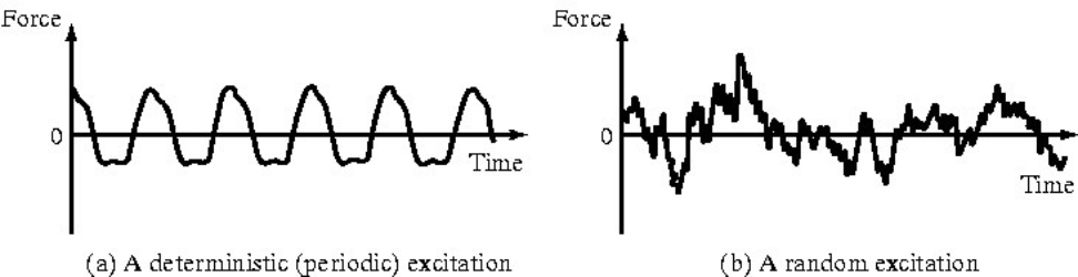
Observe the difference in the force-time histories: the deterministic plot shows a clear, periodic pattern, whereas the random excitation plot shows irregular, fluctuating values where no specific magnitude can be predicted for a future time step.

Modeling the Simple Harmonic Oscillator

To analyze any vibrational system, we must derive its governing Equation of Motion. We rely on Newton’s Second Law: F = ma. In a standard second-order system, we must account for several specific forces.

The Newtonian Sum of Forces:

• Restoration force of the spring: $-kx$
• Damping force: $-c\frac{\mathrm{d}x}{\mathrm{d}t}$
• Gravity (Weight): $W=mg$
• Static restoration force: $-k{\delta }_{st}$ (The force required to offset gravity at rest)
• External Force: $F(t)$

Synthesized Equation of Motion: When we apply $F=ma$ to a vertical mass, the sum of forces is: $m\frac{{\mathrm{d}}^{2}x}{\mathrm{d}{t}^2}=-k(x+{\delta }_{st})-c\frac{\mathrm{d}x}{\mathrm{d}t}+mg+F(t)$

In static equilibrium, the weight of the mass is perfectly balanced by the spring's static deflection force ($mg=k{\delta }_{st}$). Consequently, these terms cancel out, leaving us with the simplified dynamic equation: $m\ddot{x}+c\dot{x}+kx=F(t)$

Solving Second-Order Differential Equations

To determine the system response, we solve the homogeneous equation $m\ddot{x}+c\dot{x}+kx=0$. Engineers simplify this by writing the characteristic equation in terms of a variable $a$: $a^2+P_{1}a+P_0=0$

By solving for the roots $a_{1,2}$ using the quadratic formula, we identify 3 distinct physical behaviors:

1. Distinct Real Roots ($P_1^2\ne 4P_0$): The system is overdamped. The general solution is $y(t)=C_1{e}^{a_{1}t}+C_2{e}^{a_{2}t}$.
2. Complex Roots ($z_{1,2}=\alpha \pm i\beta$): The system is underdamped. The solution is oscillatory: $y(t)=C_1{e}^{\alpha t}\cos \beta t+C_2{e}^{\alpha t}\sin \beta t$.
3. Repeated Roots ($a_1=a_2$): The system is critically damped. The solution is $y(t)=C_1{e}^{a_{1}t}+C_{2}t{e}^{a_{1}t}$.

System Responses and Damping Characteristics

The Damping Ratio ($\zeta$) is the ratio of the actual damping coefficient ($c$) to the critical damping coefficient ($c_c$). It dictates the decay of the system:

• Overdamped ($\zeta >1$): High resistance; the mass creeps back to equilibrium without ever crossing it.
• Critically Damped ($\zeta =1$): The threshold state where the system returns to equilibrium in the shortest time possible without oscillation.
• Underdamped ($\zeta <1$): The system oscillates with diminishing amplitude. The response is described by: $x=e^{-\gamma t}a\cos [{\omega }_{1}t-\alpha ]$.

Figure 2: Simple Harmonic Oscillator.

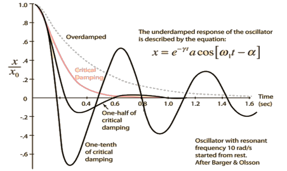
Observe the decay curves. A system with "one-tenth of critical" damping ($\zeta =0.1$) exhibits many large oscillations. As \zeta increases to "one-half of critical" ($\zeta =0.5$), the oscillations are suppressed much faster, demonstrating the efficiency of energy dissipation.

Key Takeaway: It is vital to select appropriate damping levels to avoid Aerodynamic Flutter. Without sufficient damping, aerodynamic forces can cause unstable, growing oscillations in structures like aircraft wings or bridges, leading to total structural failure.

Frequency Domain Analysis: Laplace Transforms

Engineers use the Laplace Transform to convert second-order differential equations from the time domain ($t$) into the frequency domain ($s$). This changes calculus problems into simpler algebraic ones. By defining:

• The operator $s=j\omega$
• Circular natural frequency: ${\omega }_n=\sqrt{\frac{k}{m}}$
• $\zeta =c/c_c$, actual damping / critical damping
• $c_c=2m\sqrt{\frac{k}{m}}=2m{\omega }_n$

We derive the Transfer Function, $H(s)$, representing the ratio of output $X(s)$ to input $F(s):H(s)=\frac{X(s)}{F(s)}=\frac{1}{m{s}^2+cs+k}$

To reach the standard engineering form, we normalize this into the Transfer Function $G(s)$:

$$G(s)=\frac{{\omega }_n^2}{s^2+2\zeta {\omega }_{n}s+{\omega }_n^2}$$

The frequency response can be written as

$$G(j\omega )=\frac{1}{[1-(\omega /{\omega }_n{)}^2]+j2\zeta (\omega /{\omega }_n)}$$

The magnitude is:

$$|G(j\omega )|=\frac{1}{\sqrt{[1-(\omega /{\omega }_n{)}^2{]}^2+(2\zeta (\omega /{\omega }_n){)}^2}}$$

Define the normalized frequency as ${\omega }_v=\omega /{\omega }_n$, we have the normalized magnitude $|G(j{\omega }_v)|$:

$$|G(j{\omega }_v)|=\frac{1}{\sqrt{(1-{\omega }_v^2{)}^2+(2\zeta {\omega }_v{)}^2}}$$

In the frequency domain, we analyze the Bandwidth, which is the range of frequencies over which the system responds significantly. This bandwidth varies based on the damping ratio $\zeta$ and natural frequency ${\omega }_n$.

Figure 3: Different zeta.

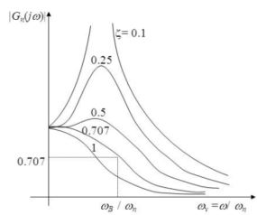
These plots illustrate resonance. As the frequency ratio $\omega /{\omega }_n$ approaches $1$, the magnitude peaks. Note that as $\zeta$ decreases, the peak magnitude becomes sharper and higher. Conversely, higher damping "flattens" the curve, reducing the peak response.

Free Vibrations of Undamped Systems

Free vibration occurs when a system oscillates purely under an initial disturbance ($x_0$ or ${\dot{x}}_0$) with no continuous external force.

Classified by damp:

• Undamped vibrations result when amplitude of motion remains constant with time (e.g., in a vacuum)
• Damped vibrations occur when the amplitude of free vibration diminishes gradually overtime, due to resistance offered by the surrounding medium (e.g., air)

Classified by system:

• The Horizontal System: Frictionless motion results in:$$m\ddot{x}+kx=0$$
• The Vertical System: As established in Section 3, gravity ($mg$) and static deflection ($k{\delta }_{st})$ cancel out, yielding the same result:$$m\ddot{x}+kx=0$$

This indicates that when a mass moves in a vertical direction, we can ignore its weight, provided we measure $x$ from its static equilibrium position.

The Euler Bridge to Harmonic Motion: We initially assume a solution in complex exponentials: $x(t)=C_1{e}^{i{\omega }_{n}t}+C_2{e}^{-i{\omega }_{n}t}$. By applying Euler’s Formula $(e^{i\varphi }=\cos \varphi +i\sin \varphi )$, we can transition to the more practical trigonometric form:

$$x(t)=A_1\cos {\omega }_{n}t+A_2\sin {\omega }_{n}t$$

Applying Initial Conditions:

$$x(t=0)=A_1=x_0,\dot{x}(t=0)={\omega }_n{A}_2={\dot{x}}_0$$

By solving for constants using initial displacement $(x_0)$ and velocity $({\dot{x}}_0)$, we find:

$$x(t)=x_0\cos {\omega }_{n}t+\frac{{\dot{x}}_0}{{\omega }_n}\sin {\omega }_{n}t$$

The motion equation and its solution are harmonic functions of time.

The motion equation $x(t)=A_1\cos {\omega }_{n}t+A_2\sin {\omega }_{n}t$ can be expressed as:

$$x(t)=A_0\sin ({\omega }_{n}t+{\varphi }_0)$$

where $A_0,{\omega }_0,{\varphi }_0$ are new constants, amplitude and phase angle respectively, and

$$A_0=A={[x_0^2+{\left(\frac{{\dot{x}}_0}{{\omega }_n}\right)}^2]}^{1/2},{\varphi }_0={\tan }^{-1}\left(\frac{x_0{\omega }_n}{{\dot{x}}_0}\right)$$

1. For vertical system, the spring constant:

$$k=\frac{W}{{\delta }_{\text{st}}}=\frac{mg}{{\delta }_{\text{st}}}$$

Hence:

$${\omega }_n={\left(\frac{g}{{\delta }_{\text{st}}}\right)}^{1/2}$$

Hence, natural frequency in cycles per second:

$$f_n=\frac{1}{2\pi }{\left(\frac{g}{{\delta }_{\text{st}}}\right)}^{1/2}$$

and, the natural period:

$${\tau }_n=\frac{1}{f_n}=2\pi {\left(\frac{{\delta }_{\text{st}}}{g}\right)}^{1/2}$$

2. Velocity $\dot{x}(t)$ and the acceleration ${\ddot{x}}_0$ of the mass $m$ at time $t$ can be obtained as:

$$\begin{array}{rl}& \dot{x}(t)=\frac{\mathrm{d}x}{\mathrm{d}t}(t)=-{\omega }_{n}A\sin ({\omega }_{n}t-\varphi )={\omega }_{n}A\cos ({\omega }_{n}t-\varphi +\pi /2)\\ & \ddot{x}(t)=\frac{{\mathrm{d}}^{2}x}{\mathrm{d}{t}^2}(t)=-{\omega }_n^{2}A\cos ({\omega }_{n}t-\varphi )={\omega }_n^{2}A\cos ({\omega }_{n}t-\varphi +\pi )\end{array}$$

• If initial displacement ($x_0$) is zero,

$$x(t)=\frac{{\dot{x}}_0}{{\omega }_n}\cos ({\omega }_{n}t-\pi /2)=\frac{{\dot{x}}_0}{{\omega }_n}\sin {\omega }_{n}t$$

• If initial velocity (${\dot{x}}_0$) is zero,

$$x(t)=x_0\cos {\omega }_{n}t$$

Free Vibration with Viscous Damping

Damping force: $F_{\text{damp}}=-c\dot{x}$, where $c$ is the damping constant.

In the vertical system, Newton’s law yields the equation of motion:

$$m\ddot{x}=-c\dot{x}-kx⟹m\ddot{x}+c\dot{x}+kx=0$$

Assume a solution in the form: $x(t)=C{e}^{st}$, where $C$ and $s$ are undetermined constants

Hence, the characteristic equation is

$$m{s}^2+cs+k=0$$

The roots of which are:

$$s_{1,2}=\frac{-c\pm \sqrt{c^2-4mk}}{2m}=-\frac{c}{2m}\pm \sqrt{{\left(\frac{c}{2m}\right)}^2-\frac{k}{m}}$$

These roots give two solutions to:

$$x_1(t)=C_1{e}^{s_{1}t},x_2(t)=C_2{e}^{s_{2}t}$$

Critical Damping Constant and Damping Ratio: The critical damping $c_c$ is defined as the value of the damping constant $c$ for which the radical in the prior becomes zero:

$${\left(\frac{c_c}{2m}\right)}^2-\frac{k}{m}=0⟹c_c=2m\sqrt{\frac{k}{m}}=2\sqrt{km}=2m{\omega }_n$$

The damping ratio $\zeta$ is defined as $\zeta =c/c_c$.

Thus, the general solution is

$$x(t)=C_1{e}^{(-\zeta +\sqrt{{\zeta }^2-1}){\omega }_{n}t}+C_2{e}^{(-\zeta -\sqrt{{\zeta }^2-1}){\omega }_{n}t}$$

Assuming that $\zeta \ne 0$, consider the following 3 cases:

• Case 1: Underdamped system ($\zeta <1,c<c_c,c/2m<\sqrt{k/m}$): For this condition, $({\zeta }^2-1)$ is negative and the roots are:

  $$\begin{array}{rl}& s_1=(-\zeta +i\sqrt{1-{\zeta }^2}){\omega }_n\\ & s_2=(-\zeta -i\sqrt{1-{\zeta }^2}){\omega }_n\end{array}$$

  and the solution can be written in different forms:

  $$\begin{array}{rl}x(t)& =C_1{e}^{(-\zeta +i\sqrt{1-{\zeta }^2}){\omega }_{n}t}+C_2{e}^{(-\zeta -i\sqrt{1-{\zeta }^2}){\omega }_{n}t}\\ & =e^{-\zeta {\omega }_{n}t}\{C_1{e}^{i\sqrt{1-{\zeta }^2}{\omega }_{n}t}+C_2{e}^{-i\sqrt{1-{\zeta }^2}{\omega }_{n}t}\}\\ & =e^{-\zeta {\omega }_{n}t}\{C_1^{\prime }\cos \sqrt{1-{\zeta }^2}{\omega }_{n}t+C_2^{\prime }\sin \sqrt{1-{\zeta }^2}{\omega }_{n}t\}\\ & =X{e}^{-\zeta {\omega }_{n}t}\sin (\sqrt{1-{\zeta }^2}{\omega }_{n}t+\varphi )\\ & =X_0{e}^{-\zeta {\omega }_{n}t}\cos (\sqrt{1-{\zeta }^2}{\omega }_{n}t-{\varphi }_0)\end{array}$$

  For the initial conditions at $t=0$:

  $$C_1^{\prime }=x_0,C_2^{\prime }=\frac{{\dot{x}}_0+\zeta {\omega }_n{x}_0}{\sqrt{1-{\zeta }^2}{\omega }_n}$$

  and hence the solution becomes

  $$x(t)=e^{-\zeta {\omega }_{n}t}\{x_0\cos (\sqrt{1-{\zeta }^2}{\omega }_{n}t)+\frac{{\dot{x}}_0+\zeta {\omega }_n{x}_0}{\sqrt{1-{\zeta }^2}{\omega }_n}\sin (\sqrt{1-{\zeta }^2}{\omega }_{n}t)\}$$

  The above equation describes a damped harmonic motion. Its amplitude decreases exponentially with time, as shown in the figure below.

  

  Figure 4: Undamped system.

  The frequency of damped vibration is:

  $${\omega }_d=\sqrt{1-{\zeta }^2}{\omega }_n$$

• Case 2: Critically damped system($\zeta =1,c=c_c,c/2m=\sqrt{k/m}$): In this case, the two roots are:

  $$s_1=s_2=-\frac{c_c}{2m}=-{\omega }_n$$

  Due to repeated roots, the solution is given by:

  $$x(t)=(C_1+C_{2}t)e^{-{\omega }_{n}t}$$

  Application of initial conditions gives:

  $$C_1=x_0,C_2={\dot{x}}_0+{\omega }_n{x}_0$$

  Thus, the solution becomes:

  $$x(t)=[x_0+({\dot{x}}_0+{\omega }_n{x}_0)t]e^{-{\omega }_{n}t}.$$

  

  Figure 5: Critical damped system.

  It can be seen that the motion represented by the above equation is aperiodic (i.e., nonperiodic). Since $e^{-{\omega }_{n}t}\to 0$ as $t\to \mathrm{\infty }$, the motion will eventually diminish to zero.

• Case 3: Overdamped system: ($\zeta >1,c>c_c,c/2m>\sqrt{k/m}$): The roots are real and distinct and are given by:

  $$\begin{array}{rl}& s_1=(-\zeta +\sqrt{{\zeta }^2-1}){\omega }_n<0\\ & s_2=(-\zeta -\sqrt{{\zeta }^2-1}){\omega }_n<0\end{array}$$

  In this case, the solution is given by:

  $$x(t)=C_1{e}^{(-\zeta +\sqrt{{\zeta }^2-1}){\omega }_{n}t}+C_2{e}^{(-\zeta -\sqrt{{\zeta }^2-1}){\omega }_{n}t}$$

  For the initial conditions at $t=0$,

  $$\begin{array}{rl}& C_1=\frac{x_0{\omega }_n(\zeta +\sqrt{{\zeta }^2-1})+{\dot{x}}_0}{2{\omega }_n\sqrt{{\zeta }^2-1}}\\ & C_2=\frac{-x_0{\omega }_n(\zeta -\sqrt{{\zeta }^2-1})-{\dot{x}}_0}{2{\omega }_n\sqrt{{\zeta }^2-1}}\end{array}$$

Energy dissipated in Viscous Damping

In a viscously damped system, the rate of change of energy with time is given by:

$$\frac{\mathrm{d}W}{\mathrm{d}t}=\text{force}\times \text{velocity}=Fv=-c{v}^2=-c{\left(\frac{\mathrm{d}x}{\mathrm{d}t}\right)}^2$$

The energy dissipated in a complete cycle is:

$$\mathrm{\Delta }W={\int }_{t=0}^{(2\pi /{\omega }_d)}c{\left(\frac{\mathrm{d}x}{\mathrm{d}t}\right)}^2\mathrm{d}t={\int }_0^{2\pi }c{X}^2{\omega }_d{\cos }^2{\omega }_{d}t\cdot \mathrm{d}({\omega }_{d}t)=\pi c{\omega }_d{X}^2.$$

If we assume simple harmonic motion: $x(t)=X\sin {\omega }_{d}t$

Advanced Harmonic Motion Concepts

To fully describe harmonic motion, we use several specific parameters:

• Natural Frequency (${\omega }_n$): The angular frequency calculated as $\sqrt{k/m}$.
• Natural Period ($T$): The time for one cycle, $T=2\pi \sqrt{m/k}$.
• Frequency ($f$): Cycles per second (Hz), $f=\frac{1}{2\pi }\sqrt{k/m}$.
• Amplitude ($A_0$): The maximum displacement, $\sqrt{x_0^2+({\dot{x}}_0/{\omega }_n{)}^2}$.
• Phase Angle ($\varphi$): The initial angle of oscillation, ${\tan }^{-1}(\frac{x_0{\omega }_n}{{\dot{x}}_0})$.