Introduction to Thermo-fluid Dynamics of Two-phase Flow

• Fundamentals of two-phase flow
  • Two-phase flow definition
• Fundamentals of computational simulation code for two-phase flow
• Fundamentals of mass, momentum, and energy conservation equations for two-phase flow
  • Homogeneous flow model, drift-flux model, two-fluid model
• Fundamentals of several constitutive equations
  • Flow regime map
  • Void fraction
  • Interfacial area concentration
  • Frictional pressure drop
  • Interfacial force
• Two-phase flow modeling

Fundamentals of two-phase flow

What is two-phase flow

Two-phase flow is composed of two immiscible mediums.

• Gas-liquid two-phase flow
• Solid-gas two-phase flow
• Solid-liquid two-phase flow
• Liquid-liquid two-phase flow

Class	Typical regimes	Geometry	Configuration	Examples
Separated flows	Film flow		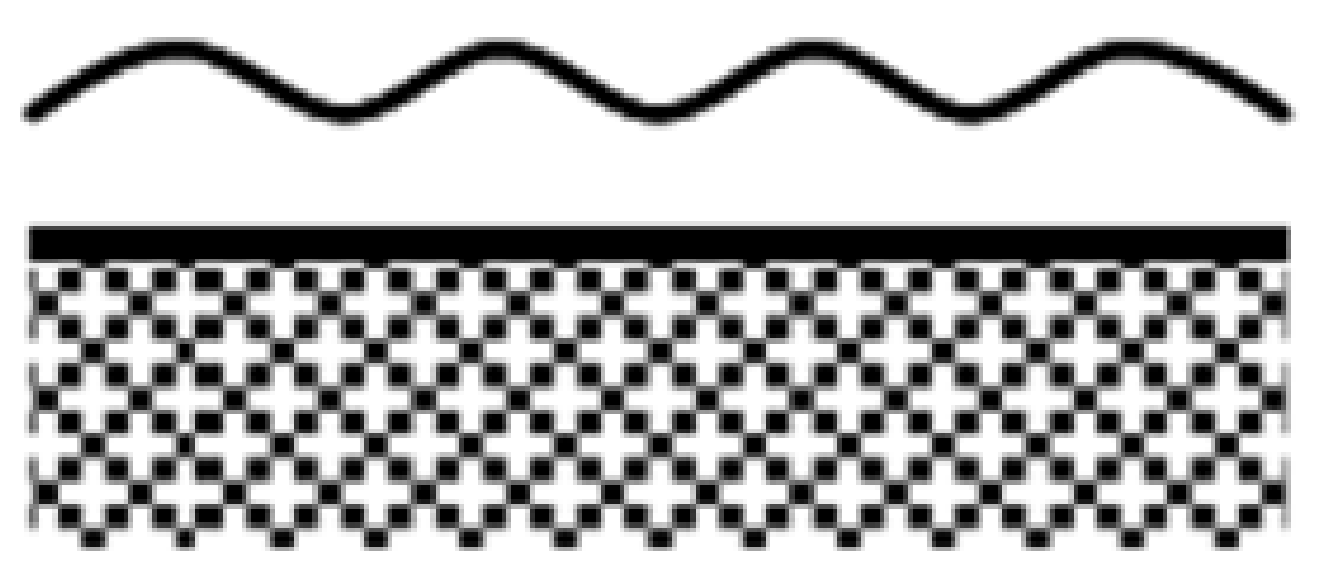Liquid film in gas; Gas film in liquid	Film condensation; Film boiling
	Annular flow		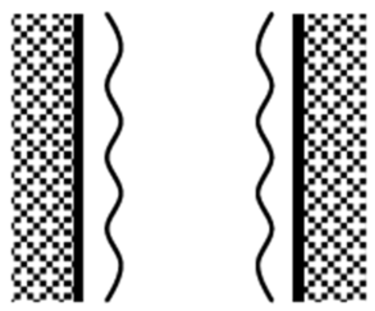Liquid core and gas film; Gas core and liquid film	Film boiling; Boilers
	Jet flow		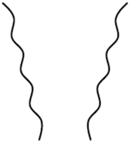Liquid jet in gas; Gas jet in liquid	Atomization; Jet condenser
Mix or Transactional flows	Cap, Slug or Churn-turbulent flow		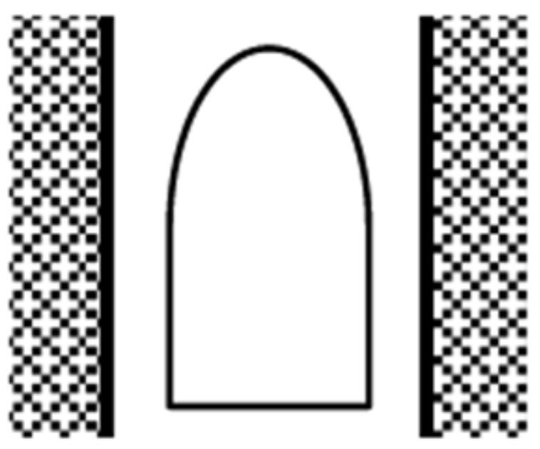Gas pocket in liquid	Sodium boiling in forced convection
	Bubbly annular flow		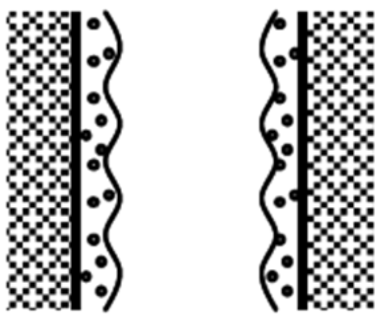Gas bubbles in liquid film with gas core	Evaporators with wall nucleation
	Droplet annular flow		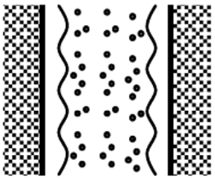Gas core with droplets and liquid film	Steam generator
	Bubbly droplet annular flow		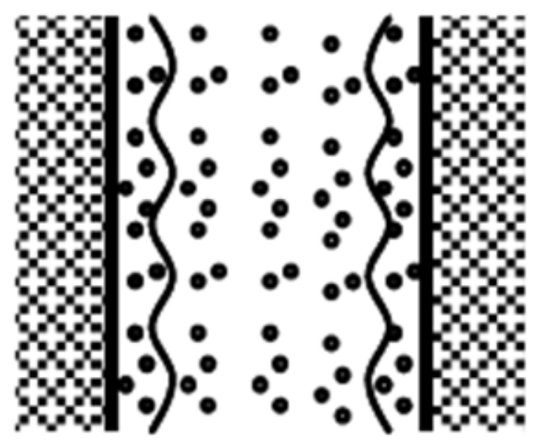Gas core with droplets and liquid film with gas bubbles	Boiling nuclear reactor channel
Dispersed flows	Bubbly flow		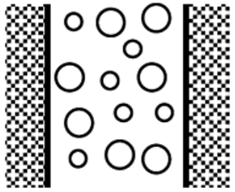Gas bubbles in liquid	Chemical reactors
	Droplet flow		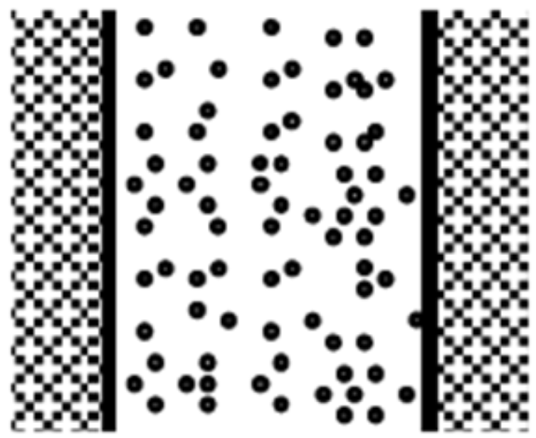Liquid droplets in gas	Spray cooling
	Particulate flow		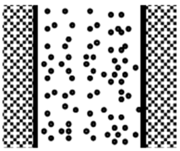Solid particles in gas or liquid	Transportaion of powder

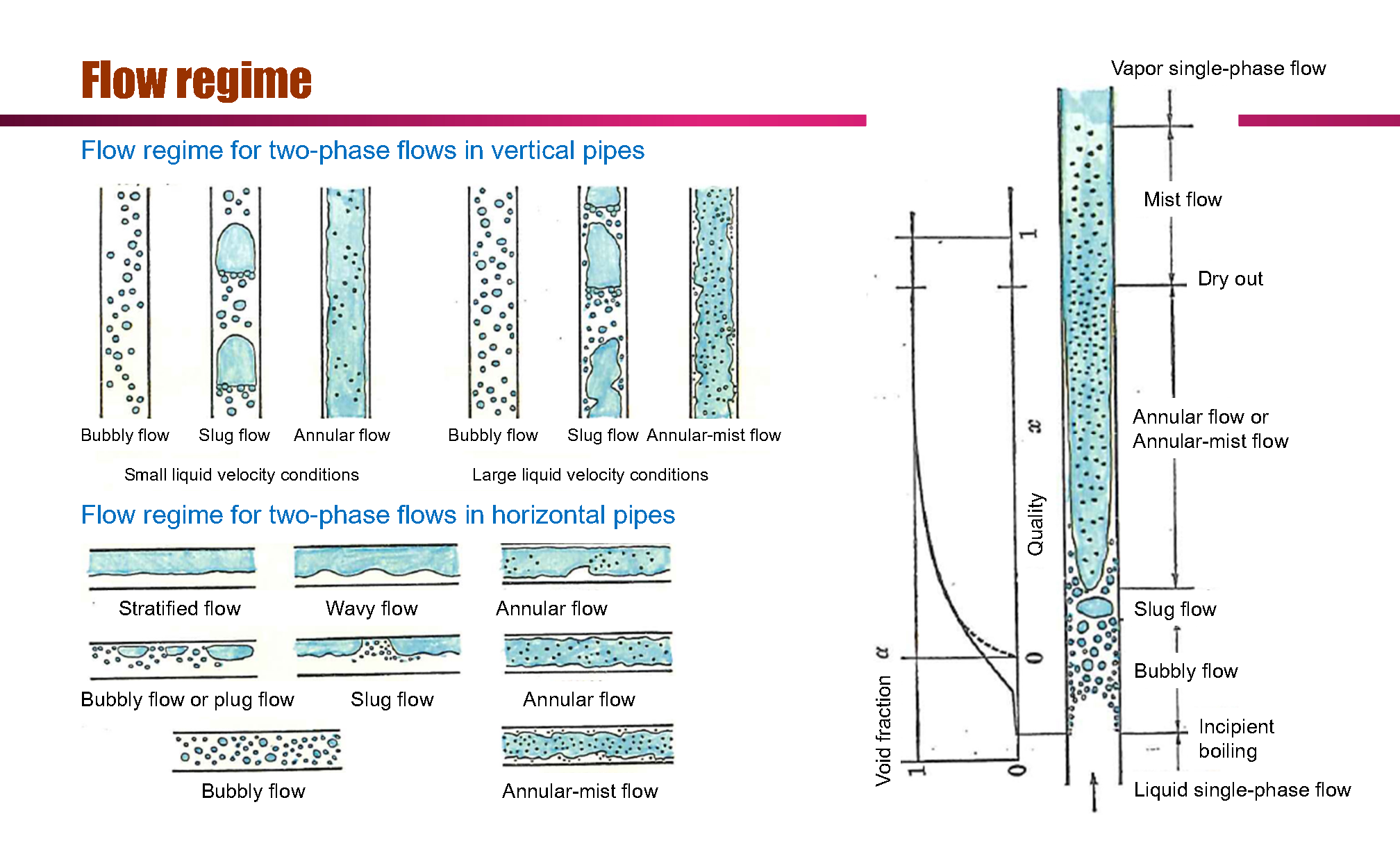
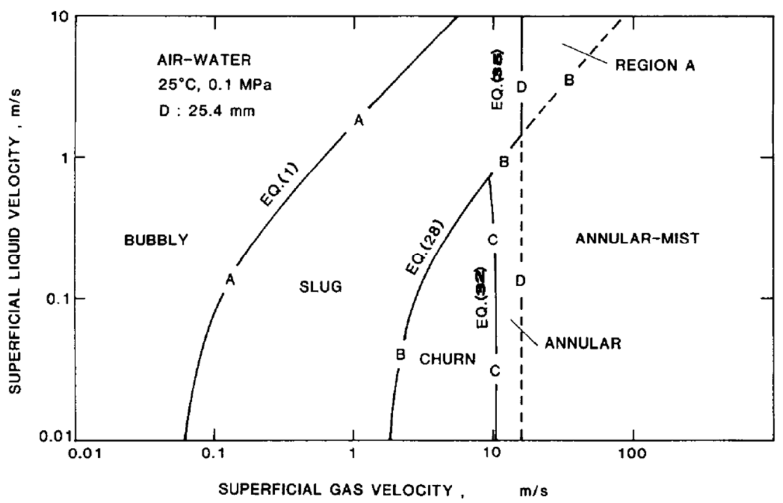
• Bubbly-to-Slug: $⟨\alpha ⟩\to 0.3$

Why is two-phase flow so difficult

Different Density:

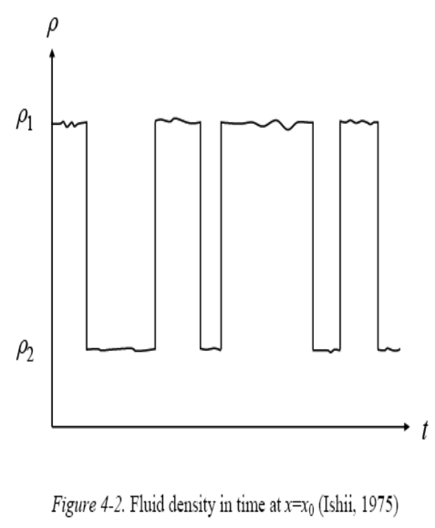
Peculiar characteristics of two-phase flow dynamics

Thermal and Kinematic Non-Equilibrium

• Driving Mechanism: Natural circulation flow, forced convective flow (laminar or turbulent flow)
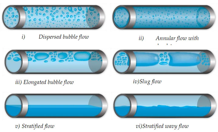
• Flow Regime: Dispersed (bubbly, slug, churn flow), separated (annular or stratified flow)
• Flow Orientation: Upward, downward, inclined, counter current, elbow, sudden expansion & contraction
• Flow Channel Scale: Micro, mini, conventional (or medium-size), large
• Phase Change: Wall nucleation & condensation, interfacial heat transfer, non-condensable gas effect
• Wall Heat Transfer: One-component with phase change, two-component without phase change
• Wall Effect: CHF, bubble nucleation, hydrophilic or hydrophobic
• Characteristic Length Scale: Kolmogorov scale, bubble size, sub-channel size, flow channel size
• Pressure and Temperature: Room temperature-to-nuclear reactor core temperature
• Gravity: Microgravity-to-elevated gravity
• Flow Instability: Geysering, chugging, density-wave oscillation
• Pressure Wave and Shock Wave: Water hammer, steam explosion
• Critical Flow: Choking flow
• Flow Structure: Internal flow, external flow
• Coupling between Two-Phase Flow & Structure: Flow induced vibration

Fundamentals of computational simulation code for two-phase flow

Key parameters in two-phase flow analysis

• Mass conservation eq.
• Momentum conservation eq.
• Energy conservation eq.

Simplified computational code structure

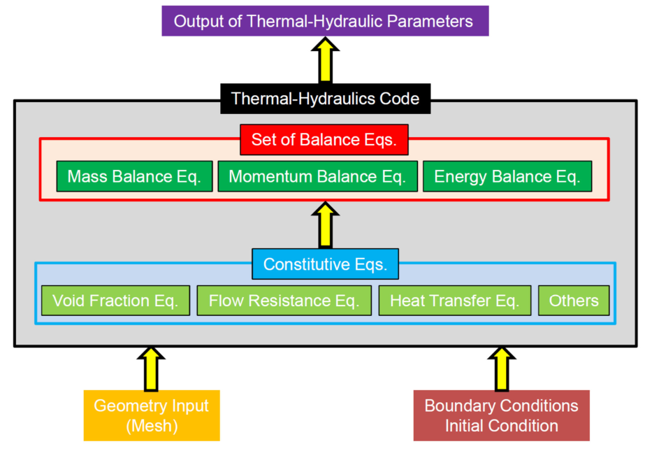
No. of balance eq. Single-phase flow: 3 Two-phase flow: 3(mixture model), 6 (=3×2), or others? Assumptions

• Relative velocity b/w gas & liquid phases
• Temperature difference b/w gas & liquid phases Two-phase flow model
• Homogeneous flow model
• Mixture model
• Two-fluid model Pros. & Cons.
• Numerical instability
• Available constitutive eqs.

Averaging methods

• Time domain
  • Instantaneous
  • Time average
• Space domain
  • Local
  • Control volume (or surface) average
  • 1D (Nuclear system analysis)
  • Porous (Steam generator analysis)
  • Sub-channel (Sub-channel analysis)
  • 3D (Detailed analysis of flow field)

Fundamentals of mass, momentum, and energy conservation equations for two-phase flow

Instantaneous single-phase flow

Reynolds number: (inertia force / viscous force)

N-S equation (Instantaneous formulation):

$$\begin{array}{rl}\rho \frac{D\mathit{v}}{Dt}=& -\mathrm{\nabla }p-\mathrm{\nabla }\cdot {\mathfrak{C}}^{\mu }+\rho \mathit{g}\\ m\mathit{a}=& \mathit{F}\end{array}$$

$\mathit{F}$ = (Surface force) + (Volumetric force)

• (Surface force) = (Pressure)+(Shear stress)
• (Volumetric force) = (Gravity)

$\mathit{a}$ = (Local acceleration) + (Convective acceleration)

Time-averaged single-phase flow

$$\begin{gathered} \overline{A\times B}\ne \overline{A}\times \overline{B} \\ \overline{A\times B}=\overline{A}\times \overline{B}+\alpha \end{gathered}$$

N-S equation (Time-averaged formulation):

$$\rho \frac{D\overline{\mathit{v}}}{Dt}=-\mathrm{\nabla }\overline{p}-\mathrm{\nabla }\cdot (\overline{{\mathfrak{C}}^{\mu }}+\underset{\text{Reynolds stress}}{\underbrace{\overline{{\mathfrak{C}}^T}}})+\rho \mathit{g}.$$

Reynolds stress: Momentum transfer due to turbulence

Turbulence models

• Mixing length model
• $k-\epsilon$ model

Time-averaged two-phase flow

Two-phase flow

• Instantaneous formulation of gas and liquid phases

$$\rho \frac{D\mathit{v}}{Dt}=-\mathrm{\nabla }p-\mathrm{\nabla }\cdot {\mathfrak{C}}^{\mu }+\rho \mathit{g}$$

• Time-averaged formulation
  • Kinematic condition (Relative velocity)
    • Homogeneous model
    • Mixture model (1 mixture momentum eq.)
      • Slip model
      • Drift-flux model
  • Two-fluid model (2 momentum eq.)
• Thermal condition (Temperature difference)
  • Thermal equilibrium (1 mixture energy eq.)
  • Thermal non-equilibrium (2 energy eq.)

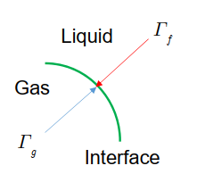
• Evaporation ($T_g>T_f$)
• Condensation ($T_g<T_f$)

Drift-flux model

4 equations:

• Mixture continuitv equation

$$\frac{\partial {\rho }_m}{\partial t}+\mathrm{\nabla }\cdot \left({\rho }_m{\mathit{v}}_m\right)=0$$

• Continuity equation for phase 2

$$\frac{\partial {\alpha }_2\overline{\stackrel{―}{{\rho }_2}}}{\partial t}+\mathrm{\nabla }\cdot \left({\alpha }_2\overline{\stackrel{―}{{\rho }_2}}{\mathit{v}}_m\right)={\mathrm{\Gamma }}_2-\mathrm{\nabla }\cdot \left({\alpha }_2\overline{\stackrel{―}{{\rho }_2}}{\mathit{V}}_{2m}\right)$$

• Mixture momentum equation

$$\frac{\partial {\rho }_m{\mathit{v}}_m}{\partial t}+\mathrm{\nabla }\cdot \left({\rho }_m{\mathit{v}}_m{\mathit{v}}_m\right)=-\mathrm{\nabla }{p}_m+\mathrm{\nabla }\cdot [\bar{\mathfrak{C}}+{\tilde{\mathfrak{C}}}^T+{\tilde{\mathfrak{C}}}^D]+{\rho }_m{\mathit{g}}_m+{\mathit{M}}_m$$

where

$$\begin{array}{rl}& {\mathfrak{C}}^D\equiv -\sum _{k=1}^2{\alpha }_k{\rho }_k{\mathit{V}}_{km}{\mathit{V}}_{km},{\mathit{V}}_{km}\equiv {\mathit{v}}_k-{\mathit{v}}_m\\ & {\mathit{v}}_m\equiv \frac{\sum _{k=1}^2{\alpha }_k{\rho }_k{\mathit{v}}_k}{{\rho }_m},{\rho }_m\equiv \sum _{k=1}^2{\alpha }_k{\rho }_k\end{array}$$

• Mixture Energy equation

$$\begin{array}{rl}& {\mathit{V}}_{kj}\equiv {\mathit{v}}_k-\mathit{j}\\ & \mathit{j}=\sum _{k=1}^2{\alpha }_k{\mathit{v}}_k\end{array}$$

Total number of unknown variables: 27: Flow regime

$$\overline{\stackrel{―}{{\rho }_k}},{\overline{\overline{p}}}_k,{\overline{\overline{T}}}_k,{\hat{i}}_k,\overline{\stackrel{―}{T_i}},\overline{\stackrel{―}{\sigma }},{\rho }_m,{\mathit{v}}_m,p_m,{\mathit{V}}_{km},\bar{\mathfrak{C}},{\mathfrak{C}}^T,{\mathit{M}}_m,{\alpha }_k,i_m,\bar{\mathit{q}},{\mathit{q}}^T,{\mathrm{\Phi }}_m^{\mu },{\mathrm{\Phi }}_m^{\sigma },{\mathrm{\Phi }}_m^i,{\mathrm{\Gamma }}_2$$

Two-fluid model [core]

Totally 6 equations:

• Continuity equation

$$\frac{\partial {\alpha }_k\overline{\stackrel{―}{{\rho }_k}}}{\partial t}+\mathrm{\nabla }\cdot \left({\alpha }_k\overline{\stackrel{―}{{\rho }_k}}\widehat{{\mathit{v}}_k}\right)={\mathrm{\Gamma }}_k$$

• Momentum equation

$$\begin{array}{rl}& \frac{\partial {\alpha }_k\overline{\stackrel{―}{{\rho }_k}}\widehat{{\mathit{v}}_k}}{\partial t}+\mathrm{\nabla }\cdot \left({\alpha }_k\overline{\stackrel{―}{{\rho }_k}}\widehat{{\mathit{v}}_k}\widehat{{\mathit{v}}_k}\right)\\ =& -\mathrm{\nabla }\left({\alpha }_k\overline{\stackrel{―}{p_k}}\right)+\mathrm{\nabla }\cdot \left[{\alpha }_k({\overline{\stackrel{―}{\mathfrak{C}}}}_k+{\mathfrak{C}}_k^T)\right]+{\alpha }_k\overline{\stackrel{―}{{\rho }_k}}{\hat{\mathit{g}}}_k+{\mathit{M}}_k\end{array}$$

• Energy equation
• 3 jump conditions

$$\sum _{k=1}^2{\mathrm{\Gamma }}_k=0\text{. }$$

Total number of unknown variables: 36: Flow regime

$${\alpha }_k,\overline{\stackrel{―}{{\rho }_k}},\widehat{{\mathit{v}}_k},{\mathrm{\Gamma }}_k,\overline{\stackrel{―}{p_k}}\stackrel{―}{\overline{{\mathfrak{C}}_k}},{\mathcal{T}}_k^T,\stackrel{―}{\overline{{\mathfrak{C}}_{ki}}},{\mathit{M}}_{ik},{\mathit{M}}_m^H,\overline{\stackrel{―}{p_{ki}}},\widehat{i_k},\stackrel{―}{\overline{{\mathit{q}}_k}},{\mathit{q}}_k^T,a_i\overline{\stackrel{―}{q_k^{\prime \prime }}}\overline{\stackrel{―}{T_k}},\overline{\stackrel{―}{T_i}},\overline{\stackrel{―}{H_{21}}},\overline{\overline{\sigma }},a_i,p^{\mathrm{s}\mathrm{a}\mathrm{t}}$$

With HEM, it becomes 3 equations

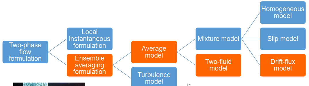
Summary of two-phase flow formulation

Fundamentals of several constitutive equations

One-dimensional computational code structure

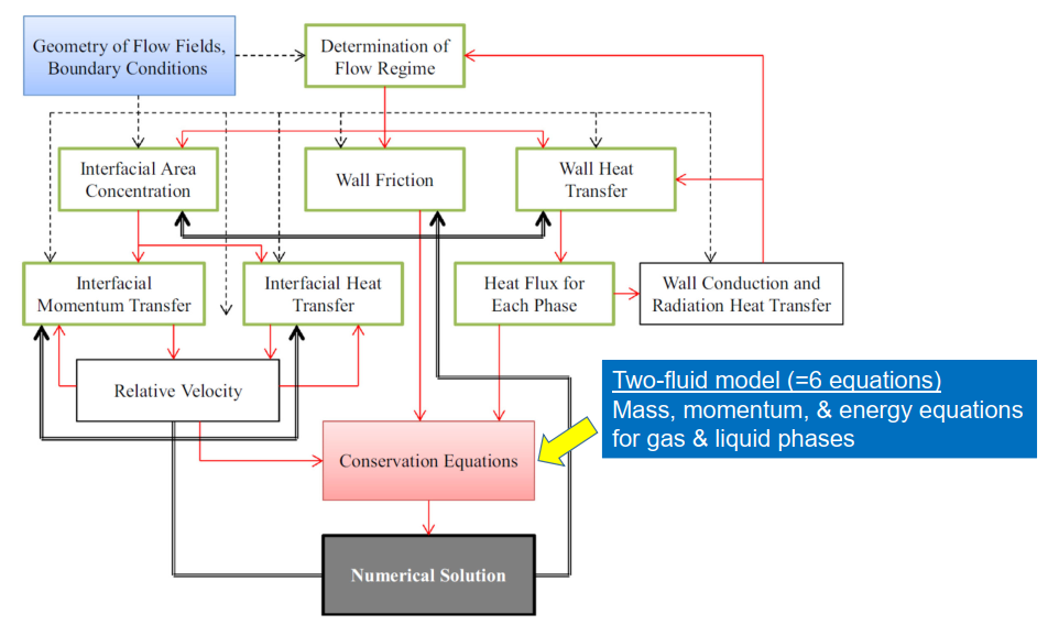
Important parameters in two-phase flow analysis [core]

• Flow regime map
  • Basic idea of flow regime transition criteria
• Void fraction
  • Basic idea of drift-flux model
• Interfacial area concentration
  • Significance of interfacial transfer terms
• Frictional pressure drop
• Interfacial force
  • Drag force
  • Non-drag force (Lift force, wall lubrication force etc.)

• scaling design
• mechanistic modeling
• instrumentation development
• experiment
• computational calculation

Flow regime map

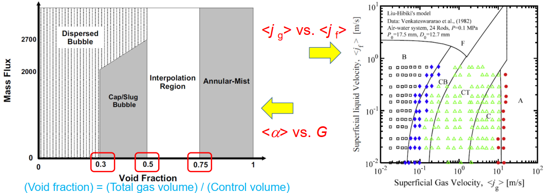
The flow regime depends on the void fraction

Void fraction

Drift velocity, which is generated by the force balance b/w buoyancy force and drag force:

$$v_{gj}=v_g-j=(1-\alpha )v_r$$

$$\begin{array}{rl}{v}_{gj}=& v_g-j=v_g-(j_g+j_f)\\ =& v_g-[\alpha v_g+(1-\alpha )v_f]\\ =& (1-\alpha )(v_g-v_f)=(1-\alpha )v_r\end{array}$$

• $⟨\cdot ⟩$: × (void fraction)
• $⟨⟨\cdot ⟩⟩$: Area-averaging

One-dimensional (or area-averaged) drift-flux model[core] :

$$⟨⟨v_g⟩⟩\equiv \frac{⟨j_g⟩}{⟨\alpha ⟩}=C_0⟨j⟩+⟨⟨v_{gj}⟩⟩$$

where $C_0$ is distribution parameter and $⟨⟨v_{gj}⟩⟩$ is the drift velocity:

$$C_0\equiv \frac{⟨\alpha j⟩}{⟨\alpha ⟩⟨j⟩},⟨⟨v_{gj}⟩⟩\equiv \frac{⟨\alpha v_{gj}⟩}{⟨\alpha ⟩}$$

$$\begin{array}{rl}& v_{gj}=v_g-j\Rightarrow \alpha v_{gj}=\alpha v_g-\alpha j\\ \Rightarrow & ⟨\alpha v_{gj}⟩=⟨\alpha v_g⟩-⟨\alpha j⟩\\ \Rightarrow & ⟨\alpha v_g⟩=⟨\alpha j⟩+⟨\alpha v_{gj}⟩\\ \Rightarrow & \frac{⟨\alpha v_g⟩}{⟨\alpha ⟩}=\frac{⟨\alpha j⟩}{⟨\alpha ⟩}+\frac{⟨\alpha v_{gj}⟩}{⟨\alpha ⟩}\\ \Rightarrow & \frac{⟨\alpha v_g⟩}{⟨\alpha ⟩}=\frac{⟨\alpha j⟩}{⟨\alpha ⟩⟨j⟩}⟨j⟩+\frac{⟨\alpha v_{gj}⟩}{⟨\alpha ⟩}\end{array}$$

In Homogeneous flow (Uniform gas distribution, $C_0=1$, & no relative velocity, $⟨⟨v_{gj}⟩⟩=0\mathrm{m}/\mathrm{s}$ ) Gas velocity:

$$⟨⟨v_g⟩⟩\equiv \frac{⟨j_g⟩}{⟨\alpha ⟩}=⟨j⟩$$

Mixture volumetric flux Center of volumetric velocity

$$⟨\alpha ⟩=\frac{⟨j_g⟩}{C_0⟨j⟩+⟨⟨v_{gj}⟩⟩}=\frac{⟨j_g⟩/⟨j⟩}{C_0+⟨⟨v_{gj}⟩⟩/⟨j⟩}$$

In HEM: $⟨⟨v_{gj}⟩⟩=0,C_0=1$

$$\begin{array}{rl}{C}_0=& \frac{⟨\alpha j⟩}{⟨\alpha ⟩⟨j⟩}\\ =& \frac{\frac{1}{A}\int \alpha j\mathrm{d}A}{\frac{1}{A}\int \alpha \mathrm{d}A\frac{1}{A}\int j\mathrm{d}A}\\ =& 1(\text{If }\alpha \text{ is constant})\end{array}$$

Distribution parameter $C_0$:

$$\{\begin{array}{ll}=1& \text{flat surface / uniform }\alpha \\ >1& \text{with surface tension}\\ <1& \text{wall peaking}\end{array}$$

Dix model for $C_0$:

$$C_0=\beta [1+{(\frac{1}{\beta }-1)}^b]$$

where

$$b={\left(\frac{{\rho }_g}{{\rho }_l}\right)}^{0.1}$$

$$\beta =\left(\frac{Gx}{{\rho }_g}\right)/(\frac{Gx}{{\rho }_g}+\frac{G(1-x)}{{\rho }_f})$$

• For regular pipe:

$$C_0=1.2-0.2{\left(\frac{{\rho }_g}{{\rho }_f}\right)}^{0.5}.$$

• For rectangular channel / duct:

$$C_0=1.35-0.35{\left(\frac{{\rho }_g}{{\rho }_f}\right)}^{0.5}.$$

• For rod bundle:

$$C_0=1.10-0.10{\left(\frac{{\rho }_g}{{\rho }_f}\right)}^{0.5}.$$

• For Subcooled boiling flow:

$$C_0=1.2-0.2{\left(\frac{{\rho }_g}{{\rho }_f}\right)}^{0.5}(1-e^{-18⟨\alpha ⟩})⟹C_0=1.2\text{ If }⟨\alpha ⟩=0.$$

$C_0$: Channel geometry dependent

Drift velocity $⟨⟨v_{gj}⟩⟩$:

Suggested by Lahey & Moody:

$$v_{gj}=2.9{\left[\left(\frac{{\rho }_f-{\rho }_g}{{\rho }_f^2}\right)\sigma g\right]}^{0.25}$$

• Bubbly:

$$⟨⟨v_{gj}⟩⟩=\sqrt{2}{\left(\frac{\mathrm{\Delta }\rho g\sigma }{{\rho }_f^2}\right)}^{1/4}(1-⟨\alpha ⟩{)}^{1.75}$$

• Slug:

$$⟨⟨v_{gj}⟩⟩=0.35{\left(\frac{\mathrm{\Delta }\rho g\sigma }{{\rho }_f^2}\right)}^{0.5}$$

• Churn:

$$⟨⟨v_{gj}⟩⟩=\sqrt{2}{\left(\frac{\mathrm{\Delta }\rho g\sigma }{{\rho }_f^2}\right)}^{1/4}$$

Development of void fraction model

1. HEM, and 20% overprediction
2. Slip model: Slip ratio $s=$

$$s=\frac{v_g}{v_f}=\frac{j_g/\alpha }{j_f/(1-\alpha )}=\frac{(1-\alpha )j_g}{\alpha j_f}\to s\frac{j_f}{j_g}=\frac{1}{\alpha }-1\to \alpha =\frac{1}{1+s\frac{j_f}{j_g}}$$

3. Drift-flux model

Interfacial area concentration

• Mass equation

$$\frac{\partial {\alpha }_k{\rho }_k}{\partial t}+\mathrm{\nabla }\cdot \left({\alpha }_k{\rho }_k{\mathit{v}}_k\right)={\overline{\mathrm{\Gamma }}}_k=a_i{m}_k$$

• Momentum equation

$$\begin{array}{rl}& \frac{\partial {\alpha }_k{\rho }_k{\mathit{v}}_k}{\partial t}+\mathrm{\nabla }\cdot \left({\alpha }_k{\rho }_k{\mathit{v}}_k{\mathit{v}}_k\right)=-{\alpha }_k\mathrm{\nabla }{p}_k+\mathrm{\nabla }\cdot {\alpha }_k({\mathfrak{C}}_k^{\mu }+{\mathfrak{C}}_k^T)\\ & +{\alpha }_k{\rho }_k\mathit{g}+{\mathit{v}}_{ki}{\mathrm{\Gamma }}_k+{\mathit{M}}_{jk}-\mathrm{\nabla }{\alpha }_k\cdot {\mathfrak{C}}_i\end{array}$$

Energy equation

$$\begin{array}{rl}& \frac{\partial {\alpha }_k{\rho }_k{H}_k}{\partial t}+\mathrm{\nabla }\cdot \left({\alpha }_k{\rho }_k{H}_k{\mathit{v}}_k\right)=-\mathrm{\nabla }\cdot {\alpha }_k({\overline{\stackrel{―}{q}}}_k+q_k^T)+{\alpha }_k\frac{D_k}{Dt}{p}_k\\ & +H_{ki}{\mathrm{\Gamma }}_k+a_i{q}_{ik}^{-1}+{\mathrm{\Phi }}_k\end{array}$$

(Interfacial transfer term)=( Interfacial area concentration ) x ( Driving potential )

$$a_i=\frac{6\alpha }{D_{\mathrm{sm}}}$$

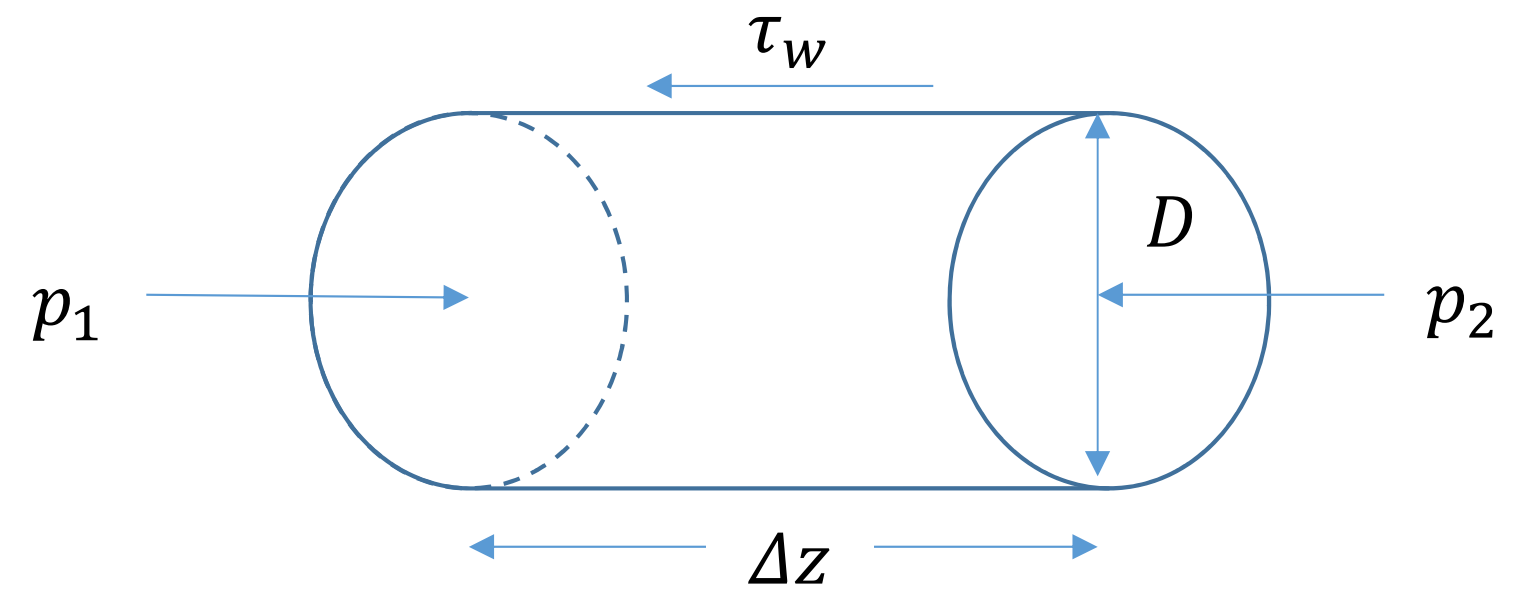
Frictional pressure drop

Lockhart-Martinelli method[core] :

$${(-\frac{\mathrm{\Delta }p}{\mathrm{\Delta }z})}_{2\varphi ,\text{fric }}={\mathrm{\Phi }}_f^2{(-\frac{\mathrm{\Delta }p}{\mathrm{\Delta }z})}_{1\varphi ,\mathrm{fric},f}\text{ Darcy friction factor }$$

where (single phase)

$${(-\frac{\mathrm{\Delta }p}{\mathrm{\Delta }z})}_{1\varphi ,\mathrm{fric},f}=\lambda \frac{1}{D}\frac{{\rho }_f{j}_f^2}{2},\lambda =\{\begin{array}{ll}64/{\mathrm{Re}}_f& \text{ for laminar flow }\\ 0.316/{\mathrm{Re}}_f^{0.25}& \text{ for turbulent flow }\end{array}$$

and $\lambda$ is Dancy friction factor; and Reynolds number:

$${\mathrm{Re}}_f\equiv \frac{{\rho }_f{j}_{f}D}{{\mu }_f}$$

For Two-phase multiplier, here's the Chiskolm equation:

$${\mathrm{\Phi }}_f^2=1+\frac{C}{X}+\frac{1}{X^2},C=20\text{for gas \& liquid turbulent flows}$$

and

$$X\equiv \sqrt{\frac{{(-\frac{\mathrm{\Delta }p}{\mathrm{\Delta }z})}_{1\varphi ,\mathrm{fric},f}}{{(-\frac{\mathrm{\Delta }p}{\mathrm{\Delta }z})}_{1\varphi ,\mathrm{fric},g}}}\text{is Martinelli parameter}$$

[Final-term]

$$\begin{array}{rl}& \pi \frac{D^2}{4}{p}_1=\pi \frac{D^2}{4}{p}_2+\pi D\mathrm{\Delta }z{\tau }_w\\ \Rightarrow & -\frac{p_2-p_1}{\mathrm{\Delta }z}=\frac{4}{D}{\tau }_w\Rightarrow -\frac{\mathrm{\Delta }p}{\mathrm{\Delta }z}=\frac{4}{D}{\tau }_w\end{array}$$

Gas	Liquid	$C$: Chisholm coefficient
Turbulent	Turbulent	20
Turbulent	Laminar	12
Laminar	Turbulent	10
Laminar	Laminar	5

$${\mathrm{Re}}_k\{\begin{array}{ll}<1000,& \text{Laminar}\\ \ge 2000,& \text{Turbulent}\end{array},k=g\text{ or }f$$

Quiz - Void fraction

Superficial gas velocity $=0.50\mathrm{m}/\mathrm{s}$, Superficial liquid velocity $=0.30\mathrm{m}/\mathrm{s}$ : What is the void fraction for air-water flow in a vertical $7\mathrm{cm}$ pipe under atmospheric pressure? Assume churn flow regime.

• Flow regime
• Flow direction
• Flow channel geometry
• Channel diameter

$$\frac{⟨j_g⟩}{⟨\alpha ⟩}=C_0⟨j⟩+⟨⟨v_{gj}⟩⟩$$

where

$$C_0=1.2-0.2\sqrt{\frac{{\rho }_g}{{\rho }_f}}=1.2$$

and

$$⟨⟨v_{gj}⟩⟩=\sqrt{2}{\left(\frac{\mathrm{\Delta }\rho g\sigma }{{\rho }_f^2}\right)}^{0.25}=0.23\mathrm{m}/\mathrm{s}$$

Thus

$$\begin{array}{rl}⟨\alpha ⟩& =\frac{⟨j_g⟩}{C_0⟨j⟩+⟨⟨v_{gj}⟩⟩}=\frac{0.50}{1.2(0.50+0.30)+0.231}=0.42\\ ⟨⟨v_g⟩⟩& =\frac{⟨j_g⟩}{⟨\alpha ⟩}=\frac{0.50}{0.42}=1.2\mathrm{m}/\mathrm{s}\end{array}$$

Quiz - Flow regime transition

Consider air-water flow in a vertical $7\mathrm{cm}$ pipe under atmospheric pressure. Derive bubbly-to-slug flow transition condition with critical void fraction of $0.30$ .

• Flow direction
• Flow channel geometry
• Channel diameter

$$\frac{⟨j_g⟩}{⟨\alpha ⟩}=C_0⟨j⟩+⟨⟨v_{gj}⟩⟩$$

where

$$\begin{array}{rl}& C_0=1.2-0.2\sqrt{\frac{{\rho }_g}{{\rho }_f}}=1.2\\ & ⟨⟨v_{gj}⟩⟩=\sqrt{2}{\left(\frac{\mathrm{\Delta }\rho g\sigma }{{\rho }_f^2}\right)}^{0.25}(1-⟨\alpha ⟩{)}^{1.75}\end{array}$$

and

$$⟨j_f⟩=\frac{1-C_0⟨\alpha {⟩}_{\text{crit }}}{C_0⟨\alpha {⟩}_{\text{crit }}}⟨j_g⟩-\frac{⟨⟨v_{gj}⟩⟩}{C_0}$$$$⟨j_f⟩=\frac{1-(1.2-0.2\sqrt{{\rho }_g/{\rho }_f})⟨\alpha {⟩}_{\text{crit }}}{(1.2-0.2\sqrt{{\rho }_g/{\rho }_f})⟨\alpha {⟩}_{\text{crit }}}⟨j_g⟩-\frac{\sqrt{2}{\left(\frac{\mathrm{\Delta }\rho g\sigma }{{\rho }_f^2}\right)}^{0.25}(1-⟨\alpha ⟩{)}^{1.75}}{(1.2-0.2\sqrt{{\rho }_g/{\rho }_f})}$$

where

$$⟨\alpha {⟩}_{\text{crit }}=0.3.$$

Quiz - Interfacial area concentration

Consider air-water flow in a vertical $7\mathrm{cm}$ pipe under atmospheric pressure. Assume the bubble size given by twice the size of Laplace length scale. Assume uniformly distributed spherical bubbles. Calculate the interfacial area concentration for bubbly flow with the void fraction of $0.20$.

$$\begin{array}{rl}& La=\sqrt{\frac{\sigma }{\mathrm{\Delta }\rho g}}=0.0027\mathrm{m}\\ & ⟨D_b⟩=2La=2\times 0.0027=0.0055\mathrm{m}\\ & ⟨\alpha ⟩=\frac{1}{6}\pi {⟨D_b⟩}^{3}n\end{array}$$

Thus

$$\begin{array}{rl}⟨a_i⟩& =\pi {⟨D_b⟩}^{2}n\\ & =\frac{6⟨\alpha ⟩}{⟨D_b⟩}=\frac{6\times 0.20}{0.0055}=220{\mathrm{m}}^{-1}\end{array}$$

Quiz2

A saturated steam-water mixture at ${290}^{\circ }\mathrm{C}$ vertically flows in a rectangular channel with a width of $40\mathrm{mm}$ and a gap length of $2.4\mathrm{mm}$ . The volumetric gas and liquid flow rates are $5.0\times {10}^{-5}{\mathrm{m}}^3/\mathrm{s}$ and $3.0\times {10}^{-5}{\mathrm{m}}^3/\mathrm{s}$, respectively. The distribution parameter is calculated by $C_0=1.35-0.35{\left({\rho }_g/{\rho }_f\right)}^{0.5}$, whereas the drift velocity is calculated by $⟨⟨v_{gj}⟩⟩=0.35{\left[\frac{({\rho }_f-{\rho }_g)g{D}_h}{{\rho }_f}\right]}^{0.5}$. The bubble Sauter mean diameter is calculated by $⟨D_{Sm}⟩=2La$. Laplace length $La$ is given by ${\left[\frac{\sigma }{({\rho }_f-{\rho }_g)g}\right]}^{0.5}$.

Here, ${\rho }_g(=39.2\mathrm{kg}/{\mathrm{m}}^3)$ and ${\rho }_f(=732\mathrm{kg}/{\mathrm{m}}^3)$ are the densities of gas and liquid, respectively. $g(=9.8\mathrm{m}/{\mathrm{s}}^2)$ is the gravitational acceleration. $D_h$ is the hydraulic equivalent diameter. $\sigma (0.0167\mathrm{N}/\mathrm{m})$ is the surface tension. Use three digits for significant digits.

1. What is the value of the distribution parameter?

$$C_0=1.35-0.35{\left(\frac{{\rho }_g}{{\rho }_f}\right)}^{0.5}=1.27.$$

$1.21-1.33$

2. What is the value of the drift velocity in $\mathrm{m}/\mathrm{s}$?

$$\begin{array}{c}{D}_h=\frac{4A}{p}=\frac{2\times 0.04\times 0.0024}{0.04+0.0024}\mathrm{m}\approx 0.00453\mathrm{m}\\ ⟨⟨v_{gj}⟩⟩=0.35{\left[\frac{({\rho }_f-{\rho }_g)g{D}_h}{{\rho }_f}\right]}^{0.5}\approx 0.0717\mathrm{m}/\mathrm{s}.\end{array}$$

$0.0681-0.0753$

3. What is the value of superficial gas velocity in $\mathrm{m}/\mathrm{s}$?

$$⟨j_g⟩=\frac{Q_g}{A}=\frac{5.0\times {10}^{-5}}{0.04\times 0.0024}\mathrm{m}/\mathrm{s}=0.521\mathrm{m}/\mathrm{s}.$$

$0.495-0.547$

4. What is the value of gas velocity in $\mathrm{m}/\mathrm{s}$?

$$\begin{array}{c}⟨j_f⟩=\frac{Q_f}{A}=\frac{3.0\times {10}^{-5}}{0.04\times 0.0024}\mathrm{m}/\mathrm{s}=0.3125\mathrm{m}/\mathrm{s}\\ \begin{array}{rl}⟨⟨v_g⟩⟩=& C_0⟨j⟩+⟨⟨v_{gj}⟩⟩=C_0(⟨j_g⟩+⟨j_f⟩)+⟨⟨v_{gj}⟩⟩\\ \approx & 1.27\times (0.521+0.3125)+0.0717\approx 1.13\mathrm{m}/\mathrm{s}.\end{array}\end{array}$$

$1.07-1.19$

5. What is the value of the void fraction?

$$⟨\alpha ⟩=\frac{⟨j_g⟩}{⟨⟨v_g⟩⟩}\approx \frac{0.521}{1.13}\approx 0.461.$$

$0.438-0.484$

6. What is the value of the bubble Sauter mean diameter in $\mathrm{m}$?

$$\begin{array}{rl}⟨D_{Sm}⟩=& 2La=2{\left[\frac{\sigma }{({\rho }_f-{\rho }_g)g}\right]}^{0.5}\\ =& 2\times \sqrt{\frac{0.0167}{(732-39.2)\times 9.8}}\mathrm{m}\approx 0.00314\mathrm{m}.\end{array}$$

$0.003-0.0033$

7. What is the value of the interfacial area concentration in $1/\mathrm{m}$?

$$a_i=\frac{6⟨\alpha ⟩}{D_{Sm}}\approx 882{\mathrm{m}}^{-1}.$$

$838-926$

8. What is the value of the two-phase mixture density in ${\mathrm{kg}/\mathrm{m}}^3$?

$$\begin{array}{rl}{\rho }_m=& ⟨\alpha ⟩{\rho }_g+(1-⟨\alpha ⟩){\rho }_f\\ =& 0.461\times 39.2+(1-0.461)\times 732\mathrm{kg}/{\mathrm{m}}^3\approx 412\mathrm{kg}/{\mathrm{m}}^3.\end{array}$$

$392-433$

9. What is the value of the two-phase mass flux in $\mathrm{kg}/{\mathrm{m}}^2\mathrm{s}$?

$$G={\rho }_g⟨j_g⟩+{\rho }_f⟨j_f⟩\approx 39.2\times 0.521+732\times 0.3125\approx 249\mathrm{kg}/{\mathrm{m}}^2\mathrm{s}.$$

$237-262$

10. What is the value of the flow quality?

$$⟨x⟩=\frac{G_g}{G}=\frac{{\rho }_g⟨j_g⟩}{G}\approx \frac{39.2\times 0.521}{249}\approx 0.0819.$$

$0.0778-0.086$