Dynamic Response of MEMS Sensors

Introduction to Sensor Dynamics

The fundamental performance of MEMS is dictated by their dynamic response to time-varying environmental inputs. In the field of high-precision sensing, understanding these temporal behaviors—particularly those governed by second-order system dynamics—is critical for ensuring signal integrity and operational stability.

This document provides a rigorous engineering overview of sensor dynamics. We will explore the mathematical foundations and physical implementations of MEMS sensing, ranging from noise analysis to complex Laplace-domain modeling.

Overall System Noise and Sensitivity Analysis

In any measurement chain, the signal of interest is inevitably accompanied by noise components that define the system's detection limits. To characterize the noise floor relative to the specific physical quantity under observation, engineers utilize standard metrics.

Commonly Used Noise Terms:

Term & Definition

• NES: Noise Equivalent Signal
• NEA: Noise Equivalent Acceleration
• NEP: Noise Equivalent Power
• NED: Noise Equivalent Displacement

Sensitivity and Signal Flow Modeling

Sensitivity is rigorously defined as the ratio of the system output noise to the responsivity. For initial steady-state characterization, we prioritize the DC signal analysis. The signal flow from a physical input acceleration (a) to a final output voltage ($V_{\text{out}}$) is modeled as follows:

$$V_{\text{out}}=(\beta a+{\delta }_{x_n})\mathcal{L}+V_n$$

In this transducer model:

• $\beta$: The Transducer gain.
• $\mathcal{L}$: The Measurement Circuit gain.
• ${\delta }_{x_n}$: Noise variables entering at the transducer stage, representing physical or mechanical noise sources.
• $V_n$: Electronic noise inherent to the measurement circuitry.

Key Takeaway: Sensitivity Variability Sensitivity is not a static parameter. It is a function of the system's bandwidth and sampling rates. Because noise levels fluctuate based on these parameters, a sensor's effective resolution will degrade as the sampling frequency increases or the filter bandwidth widens.

Core Principles of MEMS Accelerometers

Modern surface-micromachined accelerometers, such as the Analog Devices ADXL202, utilize the relationship between mechanical displacement and capacitive change to detect acceleration.

Physical Principles

The sensing mechanism is based on a proof mass ($m$) suspended by a spring system with stiffness ($K$). When subjected to acceleration ($a$), the resulting displacement ($x$) is: $x=-\frac{m}{K}a$

The displacement is detected by measuring the capacitance ($C$) between movable and fixed plates. This is governed by the parallel-plate capacitance formula: $C=\frac{\epsilon A}{d}$ where $\epsilon$ is the permittivity of the medium, $A$ is the contact (overlap) area, and $d$ is the gap distance.

Optimization for Sensitivity

To maximize accelerometer sensitivity, the mechanical design must prioritize 3 physical adjustments:

1. Increased Proof Mass ($m$): Enhances the inertial force.
2. Decreased Spring Stiffness ($K$): Reduces the restoring force, allowing for larger displacement.
3. Increased Contact Area ($A$): Increases the base capacitance and the magnitude of capacitance changes.

Mechanical Structure

The typical MEMS schematic features a proof mass—a movable microstructure—coupled to movable plates (fingers). These are interleaved with fixed outer plates. As acceleration occurs, the proof mass shifts, varying the gaps $d_1$ and $d_2$. This differential change in capacitance is then processed by the measurement circuit to determine the magnitude and direction of the input.

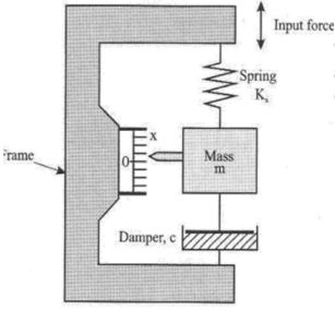
Mathematical Modeling: The Mass-Spring-Damper System

To predict the sensor’s behavior under dynamic conditions, we model the microstructure as a 2nd Order Spring-Mass-Damper system.

The Second-Order Differential Equation

The motion of the proof mass is governed by the balance of external and internal forces ($F$): $F=M\frac{{\mathrm{d}}^{2}x}{\mathrm{d}{t}^2}+D\frac{\mathrm{d}x}{\mathrm{d}t}+Kx$

• Proof mass inertia ($M\frac{{\mathrm{d}}^{2}x}{\mathrm{d}{t}^2}$): The force required to change the momentum of the mass.
• Damping force ($D\frac{\mathrm{d}x}{\mathrm{d}t}$): The energy dissipation term, usually resulting from air resistance or fluid friction.
• Mechanical restoring force ($Kx$): The linear force exerted by the springs to return the system to equilibrium.

Why it Matters The equilibrium of these forces dictates the sensor’s responsiveness. An improper balance can lead to significant lag, increased settling time, or excessive oscillation, all of which compromise the accuracy of real-time measurements.

Figure 1: mass-spring type accelerometer Flow.

Classification of Sensor Response Orders

Sensor systems are categorized by the order of the differential equation describing their input-output relationship.

Zeroth Order Systems

A zeroth-order system is an idealization where the output $y(t)$ follows the input $x(t)$ instantaneously: $y(t)=Kx(t)$.

• Pressure Sensor Example: A simple manometer where height $h=\frac{P-P_{ref}}{\rho g}$.
• Bimetal Temperature Sensor: Defined by the radius of curvature ($\rho$) of the bent beam: $\rho =\frac{t[3(1+m{)}^2+(1+mn)(m^2+\frac{1}{mn})]}{6({\alpha }_A-{\alpha }_B)(T_1-T_0)(1+m{)}^2}$ (where $n$ and $m$ are ratios of Elastic Moduli and thicknesses, and $\alpha$ is the coefficient of thermal expansion).

First Order Systems

These systems contain one energy storage element, described by the equation:

$$\begin{array}{c}{a}_1\frac{\mathrm{d}y(t)}{\mathrm{d}t}+a_{0}y(t)=x(t)\\ \frac{Y(s)}{X(s)}=\frac{K}{\tau -s+1}\end{array}$$

• Static Sensitivity ($K$): Defined as $1/a_0$.
• Time Constant ($\tau$): Defined as $a_1/a_0$. In thermal systems like thermocouples, $\tau =\frac{\rho C_{p}V}{hA}$.
• Corner Frequency (${\omega }_c$): $1/\tau$.
• Response Rules: Following a step change, the system reaches 63.2% of its steady-state value at $t=\tau$, and 95% at $t=3\tau$.

Example: Heat response

$$\frac{T-T_{\text{inf}}}{T_0-T_{\text{inf}}}=e^{-\frac{hA}{\rho C_{p}V}t}$$

Second Order Systems

Defined by two energy storage elements, governed by:

$$\begin{array}{c}{a}_2\frac{{\mathrm{d}}^{2}y(t)}{\mathrm{d}{t}^2}+a_1\frac{\mathrm{d}y(t)}{\mathrm{d}t}+a_{0}y(t)=x(t)\\ \frac{Y(s)}{X(s)}=\frac{k{\omega }_n^2}{s^2+2\xi {\omega }_{n}s+{\omega }_n^2}\end{array}$$

The dynamic performance is characterized by:

• Static Sensitivity ($k$): $1/a_0$.
• Damping Coefficient ($\xi$): $\frac{a_1}{2\sqrt{a_0{a}_2}}$.
• Natural Frequency (${\omega }_n$): $a_1/(2\sqrt{a_0{a}_2})$.

Dynamic Characteristics and Laplace Transformations

To simplify the analysis of complex measurement chains, engineers transition from the time domain (differential equations):

$$A_{0}y+A_1{y}^{(1)}+A_2{y}^{(2)}+\dots +A_n{y}^{(n)}=k(B_{0}x+B_1{x}^{(1)}+B_2{x}^{(2)}+\dots +B_m{x}^{(m)}).$$

to the complex frequency domain (algebraic equations) using the Laplace integral transformation:

$$F(s)=\mathcal{L}\{f(t)\}={\int }_0^{\mathrm{\infty }}{e}^{-st}f(t)dt.$$

where $s=\sigma +j\omega$.

It's easy to show that:

$$\mathcal{L}\left[\frac{\mathrm{d}f(t)}{\mathrm{d}t}\right]=s\mathcal{L}[f(t)]-f(0)$$

Operator Transmittance

The generalized transfer function, or operator transmittance $K(s)$, for a sensor system is expressed as: $K(s)=\frac{Y(s)}{X(s)}=k\frac{1+B_{1}s+B_2{s}^2+\cdots +B_m{s}^m}{1+A_{1}s+A_2{s}^2+\cdots +A_n{s}^n}$ This algebraic representation allows for the efficient modeling of multi-stage transducers.

Damping Response Characteristics

$$K(s)=\frac{k{\omega }_0^2}{s^2+2\beta s+{\omega }_0^2}$$

When excited by a step function, a second-order system exhibits different behaviors depending on its damping ratio. Note that in visual performance data, the parameter $\beta$ is often used to represent this damping ratio:

1. Underdamped ($\beta <1$): The system exhibits oscillations and overshoot before settling.
2. Critical Damping ($\beta =1$): The system returns to steady state in the shortest possible time without oscillation.
3. Overdamped ($\beta >1$): The system exhibits a slow, sluggish response with significant lag and no overshoot.

The Q Factor

The "Q Factor" (Quality Factor) is a dimensionless parameter related to the resonant frequency of the mechanical spring. It indicates the degree of underdamping; a high Q factor implies low energy dissipation and sustained oscillations at resonance.

$$Q=\frac{f_r}{\mathrm{\Delta }f}=\frac{{\omega }_r}{\mathrm{\Delta }\omega }$$

7. Comprehensive Technical Glossary

• $\tau$ (Time Constant): A measure of a sensor's thermal or mechanical inertia; the time required to reach 63.2% of the steady-state value.
• Static Sensitivity ($K$): The ratio of the output to the input in a steady state (1/a_0).
• Rise Time ($\mathrm{\Delta }t$): The time interval between the 10% and 90% points of the steady-state response (t_{90} - t_{10}).
• $t_{95}$: The time required to reach 95% of the steady-state response (3\tau for 1st order).
• Seebeck Effect: The physical phenomenon (temperature gradient producing voltage) that serves as the basis for thermocouple operation.
• NES/NEA/NEP/NED: Noise Equivalent Signal, Acceleration, Power, and Displacement.
• $\epsilon$: Permittivity of the dielectric medium.
• $A$: Contact area of the capacitive plates.
• $\xi$: Damping coefficient/ratio ($a_1/2\sqrt{a_0{a}_2}$).
• ${\omega }_n$: Natural frequency ($a_1/2\sqrt{a_0{a}_2}$).

Question

What is the output characteristics of a 1st order system with step input?

The output characteristics of a 1st order system (often referred to as an inertial system) when subjected to a step input are defined by an asymptotic rise toward a steady-state value without oscillation.

Key characteristics include:

1. Time-Domain Response Equation The response $y(t)$ to a unit step input is mathematically described by the following inverse Laplace transformation:

• $y(t)=k(1-e^{-t/\tau })$

In this equation:

• $k$ is the static sensitivity of the transducer, which represents the final steady-state value the output will reach.
• $\tau$ is the time constant, a measure of the system's inertia (e.g., thermal inertia for a thermometer).

2. Significant Time Milestones The system's speed and progress are quantitatively described by the time constant $\tau$:

• At $t=\tau$: The output reaches approximately 63.2% of its final steady-state value ($y(\tau )=0.6321k$).
• At $t=3\tau$: The output reaches 95% of its steady-state value.
• Rise Time ($t_{90}$): This is the time required for the output to reach 90% of its final value.

3. Transfer Function In the frequency (Laplace) domain, the behavior of a 1st order system is represented by the transfer function:

• $K(s)=\frac{Y(s)}{X(s)}=\frac{k}{1+s\tau }$

4. Physical and Electrical Analogs

• Physical Example: A thermocouple or resistance thermometer is a classic 1st order system. Its dynamic response depends on its design, material properties, and the heat transfer process.
• Electrical Analog: The 1st order response is equivalent to a simple RC circuit, where the time constant $\tau$ is equal to the product of resistance and capacitance ($RC$).

What is the output characteristics of a 2nd order system with a step or a dynamic input?

The output characteristics of a 2nd order system (often referred to as an oscillating system) depend heavily on its internal damping and the type of input received, whether a step-change or a dynamic (sinusoidal) signal. These systems typically consist of two types of energy-accumulating elements (e.g., a mass for kinetic and a spring for potential energy) and a dissipating element (e.g., a damper).

1. Response to a Step Input When a 2nd order system receives a step input, its behavior is determined by the roots of its characteristic equation, resulting in three distinct types of response:

• Overdamped: Occurs when the system has two real roots. The output approaches the steady-state value ($k$) without oscillation, appearing similar to a 1st order response but generally slower.
• Critically Damped: Occurs when the system has one real root. This represents the fastest possible response that reaches the steady-state value without any oscillation.
• Underdamped (Oscillating): Occurs when the system has two complex roots. The output oscillates around the steady-state value before eventually settling. The time-domain response for this state is mathematically described as:$$y(t)=k(1-e^{-\beta t}\sin (\omega t+\varphi ))\$\$.$$

For dynamic inputs, the output characteristics are defined by how the system reacts to different frequencies relative to its natural frequency (${\omega }_0$).

• Resonance and Magnification: In systems with low damping (high Q Factor), a resonance peak occurs near the natural frequency ($\omega /{\omega }_0=1$). At this point, the amplitude of the output is significantly magnified compared to the input.
• Frequency Dependency:
  • At low frequencies, the output accurately tracks the input with a gain near the static sensitivity ($k$).
  • As the frequency increases toward and past the natural frequency, the amplitude drops sharply, and the system acts as a low-pass filter.
• Phase Shift: The output signal will experience a phase lag relative to the input, which increases from $0^{\circ }$ at low frequencies toward $-{180}^{\circ }$ at very high frequencies.

3. Physical and Electrical Analogs

• Mechanical Analogue: A damped spring oscillator, where the spring accumulates potential energy, the mass accumulates kinetic energy, and friction dissipates energy.
• Electrical Analogue: An RLC circuit (Resistor-Inductor-Capacitor), where the inductor and capacitor accumulate energy and the resistor dissipates it.

What is the ultimate “Sensitivity” of a MEMS mechanical sensor?

The ultimate "Sensitivity" of a MEMS mechanical sensor is defined by the ratio of the system output noise to its responsivity.

Key details regarding this ultimate limit include:

• Noise Equivalent Terms: This sensitivity limit is often expressed using "noise equivalent" terms, which represent the minimum detectable signal of a specific type, such as:
  • NES: Noise Equivalent Signal
  • NEA: Noise Equivalent Acceleration
  • NEP: Noise Equivalent Power
  • NED: Noise Equivalent Displacement
• Dependency on Bandwidth: The sensitivity of a sensor is not a fixed constant; it depends on the bandwidth or sampling rate because the amount of noise present in the system varies with these parameters.
• Design for Higher Sensitivity: To improve (increase) the sensitivity of specific mechanical sensors like capacitive accelerometers, designers typically aim for a large mass ($m$), a small spring constant ($K$), and a large contact area ($A$)

Know the dynamic response characteristics of MEMS motion sensors.

MEMS motion sensors, such as accelerometers, are characterized by their behavior as 2nd order spring-mass systems. Their dynamic response defines how the sensor reacts over time and across different frequencies to physical stimuli like acceleration or vibration.

Governing Principles

The dynamic behavior of these sensors is modeled using a mass, spring, and damper model, where the relationship between the external force ($F$) and the resulting displacement ($x$) is described by a second-order differential equation:

• $F=m\frac{d^{2}x}{d{t}^2}+D\frac{dx}{dt}+Kx$
• In this system, $m$ represents the proof mass inertia, $D$ is the damping force (viscous dissipation), and $K$ is the mechanical restoring force of the spring.

Step Input Response Characteristics

When a MEMS motion sensor is subjected to a sudden step-change in input, its response is determined by its damping coefficient ($\xi$):

• Underdamped ($\xi <1$): The output oscillates around the final steady-state value before settling. Higher oscillations occur as the damping decreases .
• Critically Damped ($\xi =1$): The sensor reaches its steady-state value in the fastest possible time without any oscillation.
• Overdamped ($\xi >1$): The output approaches the steady-state value without oscillation but does so more slowly than in a critically damped system.

Frequency (Dynamic) Response Characteristics

For sinusoidal or continuous dynamic inputs, the sensor's performance depends on the frequency of the input signal relative to its natural frequency (${\omega }_0$):

• Resonance and Magnification: When the input frequency approaches the sensor's natural frequency ($\omega /{\omega }_0\approx 1$), a resonance peak occurs. The amplitude of the output is magnified, with the level of magnification governed by the "Q" Factor (Quality Factor).
• Bandwidth: The range of frequencies over which the sensor can accurately track the input is typically limited by its resonant frequency.
• Phase Shift: As the input frequency increases, the output signal develops a phase lag, moving from $0^{\circ }$ at low frequencies toward $-{180}^{\circ }$ at high frequencies.

Design for Sensitivity

To optimize a motion sensor's dynamic performance and increase its sensitivity, designers typically aim for a large proof mass ($m$) and a small spring constant ($K$). However, the ultimate sensitivity is always bounded by the system output noise relative to its responsivity.