Skip to content

MINCO: Geometrically Constrained Trajectory Optimization for Multicopters

Source: [1] Z. Wang, X. Zhou, C. Xu, and F. Gao, "Geometrically constrained trajectory optimization for multicopters", IEEE Trans. Robot., vol. 38, no. 5, pp. 3259–3278, Oct. 2022, doi: 10.1109/TRO.2022.3160022.

1 Preliminaries

1.1 Differential Flatness

Consider a dynamical system of the following type

(1)x˙=f(x)+g(x)u

with f:RnRn, g:RnRn×m, state xRn, and input uRm. The map g is assumed to have rank m. The system is said to be differentially flat, if there exists a flat output zRm determined by x and finite derivatives of u, such that x and u can both be parameterized by finite derivatives of z:

(2)x=Ψx(z,z˙,,z(s1))(3)u=Ψu(z,z˙,,z(s)),

where Ψx:(Rm)s1Rn and Ψu:(Rm)sRm are both induced by f and g. Intuitively, the state and control can be determined from z without explicit integration of the system dynamics (1).

Leveraging the flatness of a system, the trajectory generation is convenient when there are only differential constraints in (1). If we introduce a new control variable v=z(s) and denote z[s1]Rms as

(4)z[s1]=(z,z˙,,z(s1)),

the input u=Ψu(z[s1],v) then exactly linearizes the original flat system into m decoupled chains of s-integrators. Let zi denote the i-th entry in z, vi the i-th entry in v and zi[s1]=(zi,z˙i,,zi(s1)). The i-th integrator chain is

(5)z˙i[s1]=(0Is100)zi[s1]+(01)vi,

where 0 and I are a zero matrix and an identity matrix with appropriate sizes, respectively. Given an initial state and a goal state, boundary values of each integrator chain (5) can be algebraically computed. Thus any trajectory integrated from these m integrator chains can be transformed into a feasible trajectory for the original flat system via (2) and (3).

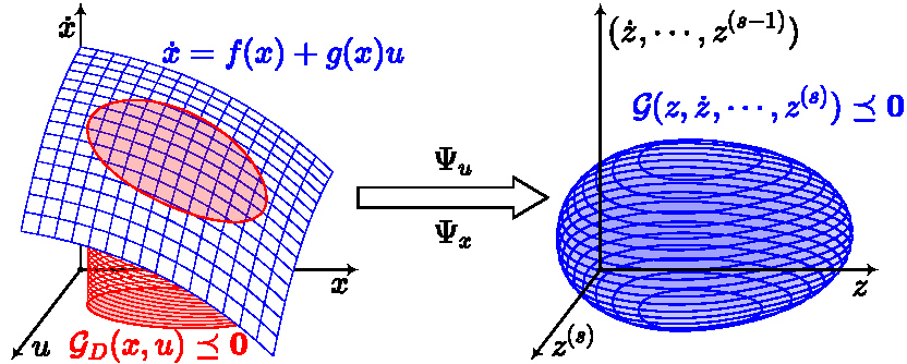
For dynamics with a small m, the flatness maps Ψx and Ψu further reduce the trajectory dimension and eliminate the differential constraints (1), which is illustrated in Fig. 1. As a side effect, nonlinearity coming from both Ψx and Ψu brings additional difficulties in trajectory generation for z when there are additional state-input constraints for (1). However, such an effect is relieved if the flat-output space coincides with the configuration space of the relevant planning problem.

fig-9-1
Figure 1[1]: Transform $\Psi_u$ and $\Psi_x$ of a flat system eliminate differential constraints (blue surface) from dynamics in the state-input space (left coordinate). The original state-input constraint $\mathcal{G}_\mathcal{D}$ (red area) is also transformed into a new constraint $\mathcal{G}$ (blue volume) in the flat-output space (right coordinate).

1.2 Direct Optimization in Flat-Output Space

Fortunately, the differential flatness of multicopters has been well studied and shown to have physically meaningful flat-output space which overlaps with the configuration space. Explicit forms of Ψx and Ψu are available in previous research (See original paper for details) for a variety of underactuated multicopters. More importantly, their flat outputs share the same form in general:

(6)z=(px,py,pz,ψ)

where (px,py,pz) is the translation of the Center of Gravity (CoG) and ψ the yaw angle of the vehicle. The flat output z, especially its translation, provides a lot of convenience for the multicopter motion planning with complex spatial constraints.

To generate feasible motions for a multicopter, we first optimize the trajectory z(t):[0,T]Rm in its flat-output space such that most of the spatial constraints are directly enforced. Then, the flatness maps Ψx and Ψu are applied to transform z(t) into the state-input trajectory x(t) and u(t).

For motion smoothness, the quadratic control effort with time regularization is adopted as a cost functional of z(t). General constraints on multicopters can be classified into configuration constraints and user-defined dynamic constraints. Normally, a collision-free motion implies

(7)z(t)F, t[0,T],

where F is the concerned obstacle-free region in configuration space. Besides, user-defined state-input constraints such as actuator limits or task-specific constraints are denoted by

(8)GD(x(t),u(t))0, t[0,T].

Exploiting Ψx and Ψu, the corresponding constraints on z(t) are computed as

(9)GD(Ψx(z[s1](t)),Ψu(z[s](t)))0, t[0,T].

Apparently, via the flatness, a constraint on x and u has its equivalent form on the finite derivatives of z(t). For simplicity, we denote (9) hereafter by

(10)G(z(t),z˙(t),,z(s)(t))0, t[0,T],

where G consists of ng equivalent constraints.

It is worth noting that we do not make further assumptions on the multicopter dynamics and flatness maps. In other words, the proposed framework supports a wide range of multicopters.

1.3 Problem Formulation

Concluding above descriptions gives the following problem:

(11a)minz(t),T0Tv(t)Wv(t)dt+ρ(T),(11b)s.t.z(s)(t)=v(t),t[0,T],(11c)G(z(t),,z(s)(t))0,t[0,T],(11d)z(t)F,t[0,T],(11e)z[s1](0)=z¯o,z[s1](T)=z¯f,

where WRm×m is a positive diagonal matrix, ρ:[0,)[0,] the time regularization, z¯oRms the initial condition and z¯fRms the terminal condition. The control input v is allowed to be discontinuous in a finite number of time instants.

The trajectory optimization (11) is nontrivial because of the continuous-time constraints G and the nonconvex set F. We further specify some reasonable conditions to make it a well-defined problem. As for time regularization ρ, it trades off between the control effort and the expectation of total time,

(12)ρs(T)=i=0MTbiTi,

where bMT is positive. Common choices are ρs(T)=kρT and ρs(T)=kρ(TTΣ)2 with an expected time TΣ. Besides, ρ can also be defined to strictly fix the total time:

(13)ρf(T)={0if T=TΣ,if TTΣ.

As for nonlinear constraints G, they are required to be C2, i.e., twice continuously differentiable. As for the feasible region F in the configuration space, we approximate it geometrically by the union of MP closed convex sets as

(14)FF~=i=1MPPi.

For simplicity, locally sequential connection is assumed on these convex sets:

(15){PiPj=if |ij|=2,Int(PiPj)if |ij|1,

where Int() means the interior of a set. The translation of z¯o and z¯f is inscribed in P1 and PMP, respectively. As for F~, we consider the case that each Pi is a closed m-dimensional ball:

(16)PiB={xRm | xoi2ri},

or, more generally, a bounded convex polytope described by its H-representation with potentially redundant constraints:

(17)PiH={xRm | Aixbi}.

For the optimization in (11), we aim to construct a computationally efficient solver while retaining the flexibility to handle different task-specific constraints GD in (8).

2 Multi-Stage Control Effort Minimization

In this section, we analyze the multi-stage control effort minimization without functional constraints.

For this problem, we propose easy-to-use optimality conditions for general cases, which are proved to be necessary and sufficient. Leveraging our conditions, the optimal trajectory is directly constructed in linear complexity of time and space, without evaluating the cost functional explicitly or implicitly.

Base on them, a novel trajectory class along with linear-complexity spatial-temporal deformation is designed to meet user-defined objectives in various trajectory planning scenarios.

2.1 Unconstrained Control Effort Minimization

When constraint F exists, adjusting the waypoints or control points of a trajectory helps to ensure safety. When constraint G exists, adjusting the time allocation also helps to enforce physical limits. Therefore, spatial and temporal parameters are both vital to a flexible trajectory representation. A natural problem is to generate a smooth trajectory subject to these parameters.

We solve Linear Quadratic Minimum-Time (LQMT) problems to generate trajectories from spatial-temporal parameters. Although the LQMT problems have extensive studies and applications, only single-stage problems are considered in the literature. We study the multi-stage problems where intermediate points and time vector are fixed in advance for multi-piece trajectories. Consider an M-stage control effort minimization without F and G,

(18a)minz(t) t0tMv(t)Wv(t) dt,(18b)s.t.  z(s)(t)=v(t), t[t0,tM],(18c) z[s1](t0)=z¯o, z[s1](tM)=z¯f,(18d) z[di1](ti)=z¯i, 1i<M,(18e) ti1<ti, 1iM.

The time interval [t0,tM] is split into M stages by M+1 fixed timestamps, with constant boundary conditions z¯o,z¯fRms. Intermediate conditions z¯iRmdi with dis specify the value of z(ti),z˙(ti),,z(di1)(ti), where di is number of derivatives fixed at ti. For example, if z(t) is only required to pass a given position at ti, then di=1 because z¯i contains the 0-order derivative and nothing else.

Existing works focus on the necessary conditions for special cases of (18). In aerial robotics area, the QP formulation and the closed-form one implicitly or explicitly optimize unknown knot derivatives, taking parameterization as a priori. This extra computation actually makes them less efficient.

In control area, a special case where di=1 is also studied via controllability Gramian. The result is for general linear systems with possibly nonpolynomial solutions while it is less intuitive considering the computational aspect. These necessary conditions can cause potential degeneracy in trajectory representation and sensitivity, if further parametric optimization on spatial-temporal parameters is needed.

2.2 Optimality Conditions

We propose necessary and sufficient optimality conditions for (18) with all possible settings of di, z¯i, and ti. Thus, an optimal trajectory can be directly constructed from spatial-temporal parameters. Furthermore, the existence and uniqueness of the optimal trajectory are always guaranteed.

We transform (18) into the Mayer form in which a new state yRms+1 augmented by y~R is defined as

(19)y=(z[s1]y~).

The augmented system y˙=f^(y,v) has the structure

(20)y˙=(A¯000)y+(0vvWv),

where

(21)A¯=(0Im(s1)0m×m0)Rms×ms.

We design a running process for the augmented system in M stages, of which the i-th is Δi=[ti1,ti]. It is worth noting that state switching occurs in this running process. Strictly speaking, the state switching only occurs on y~ at the beginning of each stage.

Denote by y[i]:ΔiRms+1 the augmented state trajectory in the i-th stage, which consists of two parts, z[i][s1] and y~[i].

At each timestamp ti, the state transfers from y[i] to y[i+1], and the part y~ is reset as

(22)y~[i+1](ti)=0, 0i<M,

thus switching the partial state from y~[i](ti) to 0.

The z[s1] part remains continuous between stages, which means

(23)z[i][s1](ti)=z[i+1][s1](ti), 1i<M.

The conditions in (18c) and (18d) are still satisfied, i.e.,

(24)z[1][s1](t0)=z¯o, z[M][s1](tM)=z¯f,(25)z[i][di1](ti)=z¯i, 1i<M.

In this process, the cost functional in (18) is converted into the sum of terminal cost of each stage for the augmented system, i.e., i=1My~[i](ti). Therefore, the optimal trajectories for the augmented system and the original one are identical in z[s1].

We utilize the Hybrid Maximum Principle to derive necessary conditions for the optimal solution.

Theorem 1: Hybrid Maximum Principle

Let t0<<tM be real numbers and Δk=[tk1,tk]. For any collection of absolute continuous functions xk:ΔkRnk, define a vector, xΣRn¯ where n¯=2k=1Mnk, as

(26)xΣ=(x1(t0),x1(t1),,xM(tM1),xM(tM)).

On the time interval Δ=[t0,tM] consider the problem

(27a)minuk,xk J(xΣ),(27b)s.t.  x˙k(t)=fk(xk(t),uk(t)),(27c) uk(t)UkRrk,(27d) tΔk, k=1,,M,(27e) η(xΣ)=0,

where fk:Rnk×RrkRnk, J:Rn¯R and η:Rn¯Rq are continuously differentiable, uk:RRrk are measurable and bounded on the corresponding Δk.

Denote an optimal process for (27) by (x(t),u(t)). Then, there exists a collection (α,γ,ψ1,,ψM), where α0, γRq and ψk:ΔkRnk are Lipschitz continuous. It generates M Pontryagin functions

(28)Hk(ψk,xk,uk)=ψkfk(xk,uk), tΔk,

and a Lagrange function L(xΣ)=αJ(xΣ)+γη(xΣ). The following conditions are satisfied for all k=1,,M.

  • Nontriviality condition:

(29)(α,γ)0;
  • Adjoint equations: for almost all tΔk,

(30)ψ˙k(t)=Hkxk(ψk(t),xk(t),uk(t));
  • Transversality conditions:

(31){ψk(tk1)=Lxk(tk1)(xΣ),ψk(tk)=Lxk(tk)(xΣ);
  • Maximality conditions: for all tΔk,

 Hk(ψk(t),xk(t),uk(t))=supukUkHk(ψk(t),xk(t),uk)(32)= 0.

Proof:

The proof can be directly adapted from Theorem 4 by Dmitruk and Kaganovich. Here we only consider each system fk to be time-invariant and all intervals Δk to be fixed. Besides, no inequality constraints are specified on xΣ.

According to Theorem 1, the costate ψ[i]:ΔiRms+1 in the i-th stage is defined as

(33)ψ[i]=(λ[i]μ[i])=(λ[i]1,λ[i]2,,λ[i]s,μ[i]),

where μ[i]:ΔiR. λ[i]j:ΔiRm is the j-th map in λ[i]:ΔiRms. The i-th Pontryagin function of (20) is

Hi(ψ[i],y[i],v[i])=ψ[i]f^(y[i],v[i])(34)=λ[i]A¯z[i][s1]+λ[i]sv[i]+μ[i]v[i]Wv[i].

By applying the adjoint equation (30) for μ[i], we have μ˙[i]=0, which means μ[i](t)=μ¯iR is a constant in Δi. Therefore, Hi is always a quadratic function of v[i],

(35)Hi(ψ[i],y[i],v[i])=λ[i]A¯z[i][s1]+λ[i]sv[i]+μ¯iv[i]Wv[i].

By applying the adjoint equation for λ[i], we obtain

(36)λ˙[i]=A¯λ[i],

which is expanded as

(37)λ˙[i]j={0if j=1,λ[i]j1if 2js.

It is obvious that λ[i]s(t) is an s1 degree polynomial.

According to maximality conditions (32), the supremum of Hi is always 0 in Δi. Thus the positive definiteness of W implies μ¯i0. If μ¯i=0, then (35) becomes a linear function of v[i]. The zero supremum means that λ[i]s(t)=0 in Δi. As the result of (36), ψ[i](t)=0 holds for all t in Δi. In such a case, a contradiction occurs that the nontriviality condition (29) and the transversality conditions (31) cannot be satisfied at the same time. Therefore, μ¯i<0 always holds in the whole Δi. The optimal control v[i] can be obtained from

(38)Hiv[i](ψ[i],y[i],v[i])=λ[i]s+2μ¯iWv[i]=0,

i.e.,

v[i](t)=12μ¯iW1λ[i]s(t), tΔi.

Then, z[i] produced by a chain of s-integrators from λ[i]s(t), is a 2s1 degree polynomial.

To further explore structures of the solution, we generate the Lagrange function using the cost of augmented system along with all constraints in (23), (24) and (25). We have

L(yΣ)= αi=1My~[i](ti)+i=0M1γiy~[i+1](ti)+ i=1M1(ζi,σi)(z[i][s1](ti)z[i+1][s1](ti))+ θo(z[1][s1](t0)z¯o)+θf(z[M][s1](tM)z¯f)(40)+ i=1M1θi(z[i][di1](ti)z¯i),

where γiR, ζiRmdi, σiRm(sdi), θoRms, θfRms and θiRmdi are all constant coefficients of corresponding constraints, yΣ is defined as in (26). Following transversality conditions (31), taking the derivative of L w.r.t. yΣ gives the boundary values of costates ψ[i] and ψ[i+1], i.e.,

(41)λ[i](ti)=(ζi+θiσi), λ[i+1](ti)=(ζiσi),(42)μ[i](ti)=μ[i+1](ti+1)=α.

Because μ[i+1](t)=μ¯i+1 in Δi+1, we have

(43)μ¯i=α, 1iM.

Finally, by substituting (36), (41) and (43) into (39), we obtain that the optimal controls of two consecutive stages satisfy

(44)v[i](j)(ti)=v[i+1](j)(ti), 0j<(sdi).

We finally know that the optimal control of the problem (18) is actually sdi1 times continuously differentiable at the timestamp ti. Accordingly, the optimal state trajectory, consisting of M polynomials with 2s1 degree, is indeed 2sdi1 times continuously differentiable at ti.

Now we conclude the conditions derived from both (39) and (44) in the following theorem, which are proved to be necessary and sufficient optimality conditions of (18).

Theorem 2: Optimality Conditions

A trajectory, denoted by z(t):[t0,tM]Rm, is optimal for the problem (18), if and only if the following conditions are satisfied:

  • The map z(t):[ti1,ti]Rm is parameterized as a 2s1 degree polynomial for any 1iM;
  • The boundary conditions in (18c);
  • The intermediate conditions in (18d);
  • z(t) is d¯i1 times continuously differentiable at ti for any 1i<M where d¯i=2sdi.

Moreover, a unique trajectory exists for these conditions.

Proof (Sketch):

Details of Proof (Sketch)

The proof of necessity is evident in the analyses from (33) to (44) that are directly derived from Theorem 1. The proof of sufficiency is sketched below:

  • The first and fourth conditions always determine a linear spline space of dimension 2s+i=1M1di for any sequence of di;
  • The second and third conditions are shown to form a square coefficient matrix on a basis of the spline space;
  • The matrix is proved to be nonsingular since ti1<ti for each i, implying the existence and uniqueness of solution;
  • The existence and uniqueness for the necessary conditions yield their sufficiency. This proof of sufficiency is detailed in Appendix of Paper (TODO).

To further explain the optimality conditions, we take the multi-stage jerk minimization as an example.

In this example, the position, velocity and acceleration are states of the jerk-controlled system (s=3). There are intermediate points (di=1) that the trajectory should pass through at certain timestamps.

The continuity of state only requires the continuity up to acceleration of the minimum-jerk trajectory, while jerk and snap of the optimal trajectory are also continuous everywhere. Accordingly, if we enforce all these continuity conditions, then Theorem 2 guarantees that only one trajectory exists, which is exactly the optimal one.

2.3 Minimization Without Cost Functional

Theorem 2 provides a direct way to construct the unique optimal trajectory. The computation enjoys linear complexity in time and space. It does not even require explicit or implicit evaluation of the cost functional or its gradient.

Consider an m-dimensional trajectory whose i-th piece is denoted by an N=2s1 degree polynomial:

(45)pi(t)=ciβ(tti1), t[ti1,ti],

where β(x)=(1,x,,xN) is the basis and ciR2s×m the coefficients. For simplicity, we use the timeline relative to t0=0. The trajectory is described by a coefficient matrix cR2Ms×m and a time vector TR>0M defined by

(46)c=(c1,,cM), T=(T1,,TM),

where Ti means the duration of the i-th piece. Then we have the timestamp ti=j=1iTj and the total duration T=T1. The M-piece trajectory p:[0,T]Rm is defined by

(47)p(t)=pi(t), t[ti1,ti), i{1,,M}.

To compute the unique solution for (18), we directly enforce optimality conditions on the coefficient matrix c. Denote by D0,DMRs×m and DiRdi×m the specified derivatives at boundaries and intermediate timestamp ti, respectively. Each column of Di is related to one dimension. Then, conditions at ti are formulated by Ei,FiR2s×2s:

(48)(EiFi)(cici+1)=(Di0d¯i×m),

Ei=(β(Ti),,β(di1)(Ti),(49)β(Ti),,β(d¯i1)(Ti)),(50)Fi=(0,β(0),,β(d¯i1)(0)).

Especially, define F0,EMRs×2s as

(51)F0=(β(0),,β(s1)(0)),(52)EM=(β(TM),,β(s1)(TM)).

The linear system for the optimal coefficient matrix is

(53)Mc=b

where MR2Ms×2Ms and bR2Ms×m are

(54)M=(F0000E1F1000E2F20000FM1000EM),

(55)b=(D0,D1,0m×d¯1,,DM1,0m×d¯M1,DM).

It is essential that the uniqueness in Theorem 2 ensures the nonsingularity of M for any time vector T0. Consequently, the unique solution c can be obtained via linear equation system (53) with a banded matrix M, i.e., a banded system.

As for a nonsingular banded system, its Banded PLU Factorization always exists, which can be employed to compute the solution with O(M) time and space complexity. Therefore, without the need of cost functional, the unique solution of problem (18) is obtained in the lowest complexity, by directly applying our optimality conditions.

2.4 MINCO Trajectories With Spatial-Temporal Deformation

For multicopters, there are often task-specific requirements apart from feasibility, such as the perception quality in active SLAM or the occlusion rate in aerial videography. These user-defined requirements majorly need to flexibly and adaptively deform both the spatial and temporal profile of a trajectory. Therefore, we select the intermediate points and the time vector as two salient parameters in (18). Fortunately, the existence and uniqueness of solution guarantee the smoothness of sensitivity for them. An iterative procedure is then designed to conduct the spatial-temporal deformation with the lowest computation complexity per iteration.

We denote the intermediate points by q=(q1,,qM1) where qiRm is a specified zero-order derivative at ti. Denote by T=(T1,,TM) the time vector where TiR>0. For any pair of q and T, Theorem 2 naturally determines a trajectory belonging to a class of control effort minimizers, named MINCO hereafter. The MINCO trajectory class, denoted by TMINCO, is defined as

TMINCO={p(t):[0,T]Rm | c=c(q,T) determined by Theorem 2,  qRm×(M1), TR>0M}.

The dimension m, the system order s, initial and terminal conditions are omitted here for brevity.

Intuitively, all trajectories in TMINCO are compactly parameterized by only q and T. Evaluating an element in TMINCO directly follows our linear-complexity formulation.

We denote any user-defined objective (or constraint) on a trajectory by a C2 function K(c,T) with available gradient. This objective on TMINCO can be computed as

(56)W(q,T)=K(c(q,T),T).

To accomplish deformation of TMINCO, the function W together with its gradient W/q and W/T are needed for a high-level optimizer to optimize the objective.

Obviously, evaluating W shares the same complexity as evaluating any trajectory in TMINCO. The key procedure is to compute the gradient.

Now we give a linear-complexity scheme to compute W/q and W/T from the given K/c and K/T. We first rewrite the linear equation system (53) as

(57)M(T)c(q,T)=b(q).

Without causing ambiguity, we omit parameters in M,b,c,K and W temporarily for simplicity. Any notation involving c is interpreted as c(q,T). Denote by qi,j the j-th entry in qi.

As for the gradient w.r.t. q, we first differentiate both sides of (57) w.r.t. qi,j, which gives

(58)cqi,j=M1bqi,j.

Then,

Wqi,j=Tr{(cqi,j)Kc}=Tr{(M1bqi,j)Kc}(59)=Tr{(bqi,j)(MKc)},

where Tr() is the trace operation.

The definition of b(q) in (55) implies that b/qi,j only has a single nonzero entry 1 at its (2i1)s+1 row and j column. Thus, stacking all the resultant scalars gives

(60)Wqi=(M1Kc)e(2i1)s+1,

where ej is the j-th column of I2Ms. Now that we have already conducted the banded PLU factorization for M when we compute c. We can reuse the factorization to avoid inverting M. Define a matrix GR2Ms×m as

(61)MG=Kc.

We only need to compute G once to obtain W/qi for all 1i<M. Denote the factorization of M as M=PLU. Specifically, L is a banded matrix with zero upper bandwidth and all-ones diagonal entries. U is a banded matrix with zero lower bandwidth and nonzero diagonal entries because of the nonsingularity of M. The pivoting matrix P simply changes the row order of the operand, satisfying PP=I. Consequently, the transpose also has a Banded LUP Factorization. Specifically, M=L¯U¯P, where

(62)L¯=U(UI)1, U¯=(IU)L,

where the inverse is only done for a diagonal matrix and the Hadamard product. Then, G can be also computed in linear complexity through such a factorization. For convenience, we partition G into

(63)G=(G0,G1,,GM1,GM)

such that G0,GMRs×m and GiR2s×m for 1i<M. After that, the gradient of W w.r.t. q is determined as

(64)Wq=(G1e1,,GM1e1),

where e1 is the first column of I2s. This operation takes out M1 specific columns in G.

As for the gradient w.r.t. T, differentiating both sides of (57) w.r.t. Ti gives

(65)MTic+McTi=0.

Thus,

WTi=KTi+Tr{(cTi)Kc}=KTiTr{(MTi)M1Kc}(66)=KTiTr{GiMTic}

The banded structure of M implies that

GMTic=GiEiTici.

Then we obtain the gradient w.r.t. Ti computed as

(68)WTi=KTiTr{GiEiTici},

where Ei/Ti can be analytically derived from (64). Computing (68) for every 1iM gives W/T.

Finally, we finish the computation of W/q and W/T. It can be verified from both (64) and (68) that the gradient propagation is also done in O(M) complexity. As for K, we make no assumption on its concrete form. Actually, the smoothness of K is not even needed if only the resultant W is C2. In other word, the linear-complexity gradient propagation enjoys both efficiency and flexibility. By incorporating it into common optimizers, we can accomplish the spatial-temporal deformation of TMINCO for a wide range of planning purposes while maintaining the local smoothness of trajectories.

3. Geometrically Constrained Flight Trajectory Optimization

In this section, we provide a unified framework for flight trajectory optimization with different time regularization ρ(T), spatial constraints F~ and continuous-time constraints G. This framework indeed relaxes the original problem into TMINCO.

The spatial-temporal deformation is utilized to meet various feasibility requirements. Lightweight schemes are specially designed to eliminate geometrical constraints such that the trajectory can be freely deformed. For continuous-time constraints, a time integral penalty functional is proposed to ensure the feasibility without sacrificing the scalability.

Finally, our framework transforms the constrained trajectory optimization into a sparse unconstrained one which can be reliably solved.

3.1 Temporal Constraint Elimination
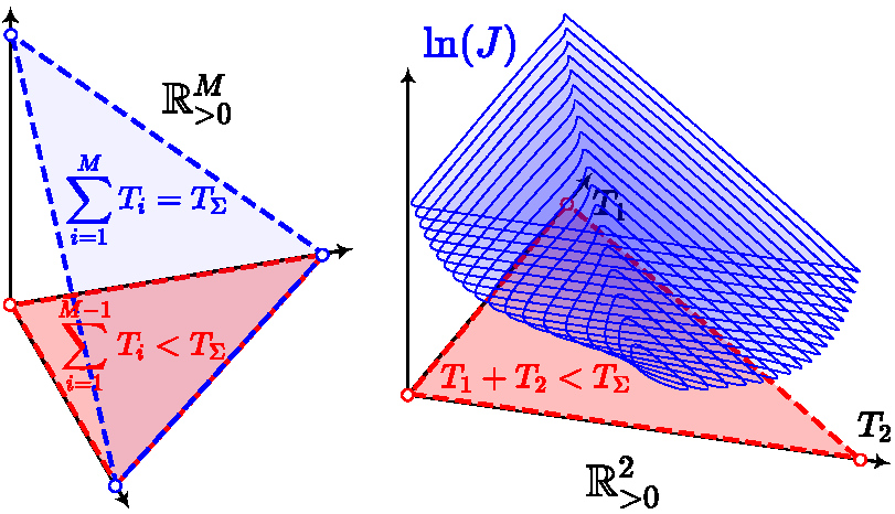
fig-9-2
Figure 2[1]: Left: Domain of $J$ on an $M$-piece trajectory with total time fixed as $T_\Sigma$. The domain is indeed the relative interior of an $(M-1)$-simplex in $\mathbb{R}^M_{>0}$. Right: Contour of $\ln{J}$ with $M=3$. The function goes to infinity as the time vector approaches the boundary of the open domain in $\mathbb{R}^2_{>0}$.

Deforming MINCO needs standard optimizers that are often designed for Euclidean spaces. However, the trajectory definition and cost functional~(11) both restrict the domain of T to simple manifolds, on which frequent retractions are needed during optimization. We give explicit diffeomorphisms for T such that surrogate variables are in Euclidean spaces. Thus, common efficient optimizers can be conveniently applied.

For polynomial splines, the control effort in (11) is a function of c and T, denoted by Jc(c,T). Analytical expressions of Jc, Jc/c, and Jc/T are available in literatures(See original paper). Now that TMINCO are polynomial splines with coefficients determined by c(q,T), the cost functional of (11) can be written as

(69)J(q,T)=Jq(q,T)+ρ(T1),

where Jq is defined as Jq(q,T)=Jc(c(q,T),T). Obviously, computing Jq, Jq/q, and Jq/T from any provided Jc, Jc/c, and Jc/T can be done in O(M) complexity, as already shown in deformation of TMINCO.

It is natural to optimize T via J/T. However, Jq(q,T) has its definition over TR>0M. It becomes unbounded when any Ti approaches zero and no consecutively repeating points appear in q. Besides, ρf defined in (13) further restricts the domain of J to i=1M1Ti<TΣ, as shown in Fig. 2.

We use diffeomorphisms to eliminate constraints for ρf and ρs. Consider the domain of ρf in (13),

(70)Tf={TRM | T1=TΣ, T0}.

It is clear that J(q,) is finite for a nontrivial q if and only if TRelInt(Tf), i.e., the relative interior of Tf.

Proposition 1:

Tf defined by (70) is diffeomorphic to RM1. Denote by τ=(τ1,,τM1) an element in RM1. A C diffeomorphism is given by the map below for 1i<M:

(71)Ti=eτi1+j=1M1eτjTΣ,  TM=TΣj=1M1Tj.

By exploiting the explicit diffeomorphism (71), we directly minimize the cost function J over RM1 via τ, because the domain constraints are satisfied by default.

Optimizing τ requires gradient propagation. We partition the gradient as Jq/T=(ga,gb), where gaRM1 and gbR.

Differentiating the layer in (71) yields the gradient of J w.r.t. τ,

(72)Jτ=(gagb1)e[τ]1+e[τ]1(gae[τ]gbe[τ]1)e[τ](1+e[τ]1)2,

where e[] is the entry-wise exponential map, and 1 an all-ones vector. If an initial guess T is specified, the corresponding τ can be computed via the inverse map of the diffeomorphism, given by τi=ln(Ti/TM) for 1i<M. As for ρs in (12), only T0 needs to be ensured. It suffices to use T=e[τ] as the diffeomorphism between RM and R>0M.

For either ρf or ρs, we denote the diffeomorphism by T(τ). Unconstrained optimization on τ can be directly conducted to minimize J(q,T(τ)). Although T(τ) does not preserve convexity, the original cost J(q,T) is already nonconvex as given in (57).

Thus, the only concern is whether T(τ) brings new local minima in the space of τ or eliminates local minima in the space of T.

Proposition 2

Denote by F:DFR any C2 function with a convex open domain DFRN. Given any C2 diffeomorphism G:RNDF, define H:RNR as H(y)=F(G(y)) for yRN. For any xDF and yRN satisfying x=G(y) or equivalently y=G1(x), the following statements always hold:

  • F(x)=0 if and only if H(y)=0;
  • 2F(x) is positive-definite (or positive-semidefinite) at F(x)=0, if and only if 2H(y) is positive-definite (or positive-semidefinite) at H(y)=0.

Proof: See Appendix in the original paper.

Proposition 2 confirms that T(τ) preserves the first/second-order necessary optimality conditions and second-order sufficient optimality conditions. It is also applicable to substitute the exponential map in this subsection with any C2 diffeomorphism from R to R>0 for a better numerical condition. In the sense of commonly-used optimality conditions, our constraint elimination does not produce extra spurious local minima or cancel any existing one.

3.2 Spherical Spatial Constraint Elimination
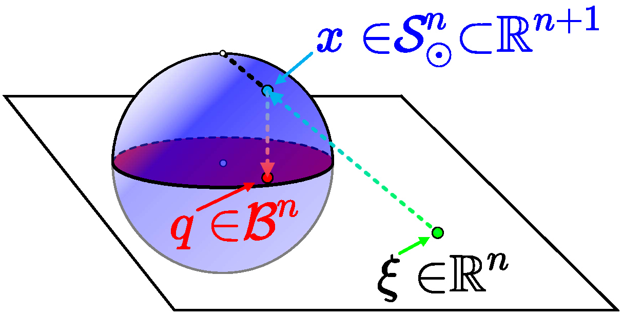
fig-9-3
Figure 3[1]: Inverse stereographic projection $f_s$ maps the Euclidean space $\mathbb{R}^n$ onto a sphere without north pole $\mathcal{S}^n_\odot$ in an $(n+1)$-dimensional space. The orthographic projection $f_o$ maps $\mathcal{S}^n_\odot$ onto an $n$-dimensional ball $\mathcal{B}^n$. The variable $\xi$ moves freely in $\mathbb{R}^n$ while the transformed variable $q$ stays in $\mathcal{B}^n$. Optimization on $\xi$ becomes unconstrained when $q$ is constrained by a ball.

We enforce motion safety by confining trajectories into the feasible region F~. Although F~ is nonconvex, it is a union of convex primitives that are sequentially connected. If all pieces have been assigned into these primitives, the safety constraint on each piece becomes convex and thus can be conveniently encoded in G. Owing to the feature of MINCO, the traverse time for every primitive can be directly optimized. Thus, we fix the piece assignment before optimization, rather than resorting to integer variables during optimization. Consequently, intermediate points should be contained by the overlap between primitives, forming inequalities. For Inequality Constrained Problems (ICPs), general methods successively approximate the constraints via additional parameters. However, we aim to apply the constraints directly and efficiently. Therefore, we propose spatial constraint elimination to enforce them exactly, leveraging their geometrical properties.

Consider the constraint qPRn where P is a closed ball. Its dimension satisfies nm since a low-dimensional constraint also exists in Rm. If P is a closed ball PB centered at point o with radius r,

(73)PB={xRn | xo2r},

We utilize a smooth surjection to map Rn to PB such that optimization over Rn implicitly satisfies the constraint PB. As illustrated in Fig. 3, the map is a composition of the inverse stereographic projection and the orthographic projection. First, we utilize the inverse stereographic projection to map Rn to Sn, where Sn is a unit sphere without north pole, i.e.,

(74)Sn={xRn+1 | x2=1, xn+1<1}.

The inverse stereographic projection fs is define as

(75)fs(x)=(2x,xx1)xx+1Sn, xRn.

Note that fs is a diffeomorphism between Rn and Sn. We then project Sn from Rn+1 back in Rn to obtain

(76)Bn={xRn | x21}.

The map is described by

(77)fo(x)=(x1,,xn)Bn, xSn,

which is indeed a smooth surjection onto Bn. Each point in Bn, except the center, is paired with two points in Sn. The composition of fs, fo, and a linear transformation, is a smooth surjection:

(78)fB(x)=o+2rxxx+1PB, xRn.

The map fB introduces a new coordinate, denoted by ξ, such that optimizing ξ over Rn always satisfies the constraint on q described by PB. For the i-th intermediate point qi, denote by ξi the corresponding new coordinate.

Accordingly, denote by ξ the new coordinate for q. Optimizing ξ requires gradient propagation for J/q.

Denote by gi the i-th entry J/qi in J/q. Differentiating the layer fB gives the gradient

(79)Jξi=2rigiξiξi+14ri(ξigi)ξi(ξiξi+1)2.

If the optimization needs to start from an initial guess q, the backward evaluation of ξ can be done by using a local inverse of fB, given by ξi for 1i<M:
(80)ξi=riri2qioi22qioi22(qioi).
fig-9-4
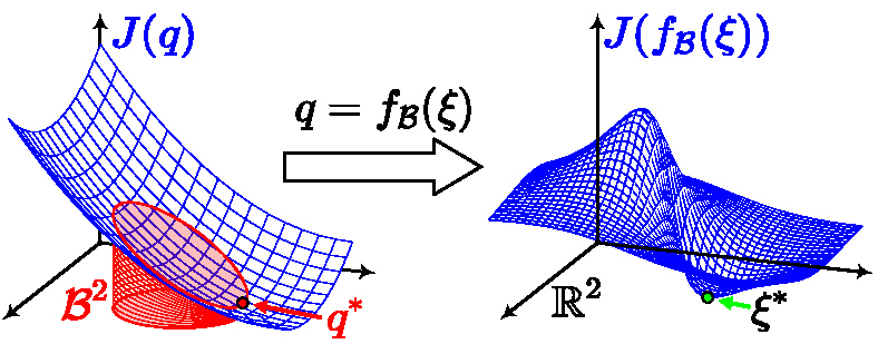
Figure 4[1]: Constrained minimum $q^*$ of a convex function $J(q)$ within a 2-D ball. Transformed by $f_\mathcal{B}$, the resultant function $J(f_\mathcal{B}(\xi))$ becomes nonconvex but it preserves the local minimum $\xi^*$ satisfying $q^*=f_\mathcal{B}(\xi^*)$ with no additional local minimum introduced.

Similarly, we analyze influences that the smooth surjection fB imposes on the constrained local minima in PB. Although fB lacks the one-to-one correspondence as diffeomorphisms possess, its components are all well-formed. Firstly, fo only takes the first n entries of a point. This operation preserves at least the first-order necessary conditions for local minima in either Bn or Sn. Secondly, fs is a diffeomorphism between Sn and Rn, thus satisfying Proposition 2. Therefore, we can also confirm that fB does not produce extra spurious local minima or cancel any existing one. As shown in Fig. 4, the constrained minimum within a 2-D ball is transformed into an unconstrained minimum.

3.3 Polyhedral Spatial Constraint Elimination
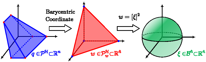
fig-9-5
Figure 5[1]: Transformations on a convex polytope. A convex polytope $\mathcal{P}^\mathcal{H}$ with $\hat{n}+1$ vertices is indeed a standard $\hat{n}$-simplex in the barycentric coordinate. The simplex $\mathcal{P}^\mathcal{H}_w$ is then the image of an entry-wise square map $[\cdot]^2$ with ball-shaped domain, which can be eliminated as in Fig. 3.

Now we consider the elimination of polyhedral constraints. Specifically, P is a closed convex polytope PH defined by

(81)PH={xRn | Axb}.

where Int(PH) according to (15). Common optimization algorithms use the H-representation of PH as linear inequality constraints. In our framework, we exploit their geometrical property to eliminate these constraints so that TMINCO can be freely deformed.

To achieve this, we use the V-representation of PH instead, where any qPH has a (general) barycentric coordinate, i.e., a convex combination of vertices. To obtain the vertices, we apply the efficient convex hull algorithm to the dual of PH based on an interior point calculated by Seidel's algorithm. Note that this procedure produces negligible overhead in our case (n4).

The procedure to eliminate a polytope constraint is illustrated in the Fig. 5. We denote all n^+1 vertices of PH by (v0,,vn^), where viRn for each i. The barycentric coordinate of a point qPH consists of the weights for these vertices. To obtain a more compact form, define v^i=viv0 and V^=(v^1,,v^n^), then the position can be calculated as

(82)q=v0+V^w,

where w=(w1,,wn^)Rn^ is the last n^ entries in the barycentric coordinate. The set of coordinates in convex combinations can also be written as

(83)PwH={wRn^ | w0, w11}.

The Main Theorem of Polytope Theory confirms the equivalence between PwH and PH under (82). The polytope is exactly converted into a standard (n^+1)-simplex by simply adding auxiliary variables and applying a linear map to q.

This process does not produce additional nonlinearity in the optimization problem except that the dimension of decision variables is increased. Therefore, we only consider the decision variables on q as the corresponding w hereafter.

The simplex (83) can be eliminated by nonlinear transformations. We first use an entry-wise square map []2:Rn^Rn^ to eliminate nonnegativity constraints using w=[x]2. Then, the constraint PwH on w is transformed into a closed unit ball Bn^ on x,

(84)Bn^={xRn^ | x21}.

Consequently, we can utilize the smooth surjection fB in (78) again. The composition of (82), []2, and fB yields a smooth surjection fH from Rn^ onto PH:

(85)fH(x)=v0+4V^[x]2(xx+1)2PH, xRn^.

A new coordinate ξ is introduced by fH, where any ξRn^ ensures qPH. The boundary of PH is also attainable. Similarly, ξ is the new coordinate for q. Optimizing ξ requires gradient propagation. Denote by gi the i-th gradient J/qi in J/q, then differentiating the layer fH gives

(86)Jξi=8ξiV^gi(ξiξi+1)216giV^[ξi]2(ξiξi+1)3ξi.

If an initial guess q is specified, the corresponding ξ can be computed via the local inverse of fH. The barycentric coordinate of each qi can be obtained using the analytic approach by Warren et al.. After that the analytic local inverses of []2 and fB() give us the desired ξi. Another flexible way is to directly minimize the squared distance between fH(ξ) and the given qi. Both approaches have negligible time consumption but promising results.

The map []2 in fH presents additional nonlinearity into optimization. Fortunately, variable transformation via []2 is a special case of the inequality-to-equality conversion. Concretely, the inequality constraints are w0. By introducing additional variables x, the equivalent equality constraints are w+[x]2=0, yielding w=[x]2. Such type of constraint conversion is proved to preserve first/second-order necessary conditions and second-order sufficient conditions for ICPs by Bertsekas as provided in literature. We confirm that the additional nonlinearity in fH does not exclude the desired minimum or produce undesired minimum practically.

Direct constraints on q are eliminated for either PB or PH using a smooth surjection q(ξ). We can conduct unconstrained optimization on ξ to minimize J(q(ξ),T(τ)) hereafter.

3.4 Time Integral Penalty Functional

After eliminating direct constraints, TMINCO can be freely deformed to meet the continuous-time constraints G. However, enforcing G over the entire trajectory involves infinitely many inequalities that cannot be solved by constrained optimization. It further needs temporal discretization that usually produces a large number of decision variables. To preserve the sparsity of trajectory parameterization, we decouple the resolution of constraint evaluation from the number of decision variables. Inspired by the constraint transcription, we transform G into finite constraints by integral of constraint violations.

For a trajectory p:[0,T]Rm, we define

(87)IGk[p]=0Tmax[G(p(t),,p(s)(t)),0]k  dt,

where kR>0 and max[,0]k is the composition of the entry-wise maximum and an entry-wise power function. Specifically, smoothing is needed if k1. The functional-type constraint is then equivalent to equality constraints IGk[p]=0. Actually, IGk[p] is a function of trajectory parameters, which we adopt as penalty terms. If k=1, it forms a nonsmooth but exact penalty. If k>1, it forms a differentiable strictly convex penalty. Thus either IG3[p] or a smoothing approximation of IG1[p] can be adopted. For simplicity, we utilize IG3[p] hereafter unless otherwise specified. There are two reasons for choosing a penalty function method. Firstly, the integral in (87) can only be evaluated numerically, making the constraint approximation inevitable.

Secondly, penalty methods have no requirement on a feasible initial guess which is nontrivial to construct.

We define the time integral penalty functional for p(t) as

(88)IG[p]=χIGk[p].

where χR0ng is a weight vector. Normally, χ should contain large constants. If no constraint is violated, IG[p] remains zero. Otherwise, if any part on p(t) violates any constraint in G, the penalty functional IG[p] grows rapidly. By incorporating IG[p] into the cost functional, continuous-time constraints are enforced within an acceptable tolerance.

Practically, IG[p] can only be evaluated by quadrature. To conduct the quadrature, we first define a sampled function Gτ:R2s×m×R>0×[0,1]Rng as

(89)Gτ(ci,Ti,τ)=G(ciβ(Tiτ),,ciβ(s)(Tiτ)),

where τ[0,1] is a normalized stamp. Then the quadrature for IG[p], denoted by I:R2Ms×m×R>0MR>0, is computed as a weighted sum of the sampled penalty,

(90)I(c,T)=i=1MTiκij=0κiω¯jχmax[Gτ(ci,Ti,jκi),0]k,

where κi controls the resolution. We choose the trapezoidal rule (ω¯0,ω¯1,,ω¯κi1,ω¯κi)=(1/2,1,,1,1/2) because of its reliable performance for ill-shaped C2 integrands in our practice. Intuitively, I(c,T) is a differentiable approximation to IG[p], whose precision is adjustable through κi. The value and gradient at most timestamps can be parallelly computed then directly combined as one.

3.5 Trajectory Optimization via Unconstrained NLP

Due to G and F in (11), the optimal trajectory parameterization is generally hard to know. Unlike traditional methods approximating solutions via a large number of variables, we propose to solve a lightweight relaxed optimization via unconstrained NLP, where the spatial-temporal deformation of TMINCO is applied. The relaxation to (11) is defined as

(91)minξ,τ J(q(ξ),T(τ))+I(c(q(ξ),T(τ)),T(τ)),

where J is the time-regularized control effort (69) for TMINCO and I is the quadrature of penalty functional (90). Note that any task-specific requirement, either objectives or constraints, can be combined in (91) without affecting its structure.

To generate trajectories for a flat multicopter, we first parameterize its flat-output trajectory as TMINCO. After assigning a fixed number of pieces into each Pi, variable transformations are applied to eliminate all direct constraints.

User-defined GD are also transformed into G via Ψx and Ψu. Finally, we obtain the cost function (91).

Apparently, the gradient propagation is derived for all layers except Ψx and Ψu. One can either apply Automatic Differentiation (AD) to Ψx and Ψu or derive the gradient propagation analytically by following the reverse-mode AD. The efficiency is the same as the flatness map as ensured by Baur-Strassen Theorem. The differentiation is only needed for the given flat dynamics once and for all. With available gradient, the relaxation (91) is then solved by the L-BFGS algorithm.

4 Conclusion (By GPT-5.2 in Github Copilot)

MINCO can be viewed as a back-end trajectory generator + lightweight unconstrained optimizer: given a piece assignment and boundary/intermediate conditions, it constructs the unique minimum-control-effort spline (solving a multi-stage LQMT like (18)), and then deforms its spatial and temporal parameters to satisfy geometry and continuous-time constraints (relaxing the original problem (11) into an unconstrained NLP (91)).

Below is a practical procedure you can follow to implement the MINCO pipeline.

MINCO procedure (implementation-oriented)

Inputs

  • Flatness order s (e.g., jerk s=3 or snap s=4), weights W, and time regularization ρ() in (11), (12), (13).
  • Start/goal boundary derivatives z¯o,z¯f (see (11e)).
  • Free-space approximation F~=iPi (see (14)(17)), plus piece assignment (e.g., K pieces per primitive).
  • Continuous-time dynamic constraints G (obtained from GD via flatness maps, see (9)(10)).

Decision variables

  • Spatial variables ξ that generate intermediate points q(ξ) using a smooth surjection (e.g., ball case (78), polytope case via fH).
  • Time variables τ that generate T(τ) via a diffeomorphism (e.g., fixed-sum case (71); gradient uses (72)).

Algorithm

  1. Discretize the topology (piece assignment)

    • Choose M polynomial pieces and assign each piece to a convex primitive Pi (sequential connection as in (15)).
    • Define intermediate points {qi} that must lie in overlaps of adjacent primitives (handled later by the surjection q(ξ)).
  2. Parameterize the flat-output trajectory as a MINCO spline

    • Represent each piece with polynomial coefficients ci and duration Ti.
    • Use the MINCO construction to obtain coefficients from spatial-temporal parameters: c=c(q,T) (banded linear system such as (57)).
    • Compute the smoothness+time costJ(q,T)=Jq(q,T)+ρ(T1)(69).
  3. Eliminate direct constraints by variable transformations

    • Time positivity / fixed total time: optimize over τ and map to T(τ) (e.g., (71)).
    • Geometry of intermediate points: optimize over ξ and map to q(ξ) (e.g., (78) for balls; analogous smooth surjection for polytopes).
    • After this step, constraints like T0 and qiP are satisfied by construction.
  4. Handle continuous-time constraints via integral penalty

    • Convert the infinite constraints G(z(t),,z(s)(t))0 into a penalty functional (87)(88).
    • Numerically evaluate it by quadrature, yielding I(c,T) in (90).
  5. Solve the unconstrained NLP

    • Minimize the relaxed objectiveminξ,τJ(q(ξ),T(τ))+I(c(q(ξ),T(τ)),T(τ))(91).
    • Use L-BFGS (as described at the end of §3.5). For gradients, propagate through layers:
      • MINCO layer c(q,T): linear-complexity gradients w.r.t. q and T (see (64), (68)).
      • Time map T(τ): use (72) (or the exponential map case).
      • Spatial map q(ξ): use the analytic Jacobians (e.g., (86)).
      • Flatness maps Ψx,Ψu: use AD or derive reverse-mode gradients once (see §3.5).
  6. Recover the feasible multicopter trajectory

    • Output the optimized flat trajectory z(t), then map to state/input using (2)(3).
    • Validate z(t)F and G0 using the same sampling resolution κi as in (90).

This procedure is exactly the “MINCO-as-a-module” viewpoint: (i) construct the unique minimum-effort spline from q,T, and (ii) optimize q,T (via ξ,τ) to satisfy geometry and dynamics.

Released under the MIT License.