Introduction to Linear Partial Differential Equations*

This is the note from MNE8108 Engineering Methods in the Department of Mechanical Engineering, CityU (semester A, 2025)

Contents mostly From Advanced Calculus for Applications by Francis Begnaud Hildebrand

Partial differential equations definition

Motivation

Why do we study partial deferential equations (PDEs) and analytic solutions?

We are interested in PDEs because most of mathematical physics is described by such equations. For example, fluids dynamics (and more generally continuous media dynamics), electromagnetic theory, quantum mechanics and etc.

Typically, a given PDE will only be accessible to numerical solution and analytic solutions in a practical or research scenario are often impossible. However, it is vital to understand the general theory in order to conduct a sensible investigation. For example, we may need to understand what type of PDE we have to ensure the numerical solution is valid. Indeed, certain types of equations need appropriate boundary conditions; without a knowledge of the general theory it is possible that the problem may be ill-posed and the solution is erroneous.

Definition

Definition: Partial derivatives

Partial derivatives: The differential (or differential form) of a function $f$ of $n$ independent variables, $(x_1,x_2,\dots ,x_n)$, is a linear combination of the basis form $(\mathrm{d}{x}_1,\mathrm{d}{x}_2,\dots ,\mathrm{d}{x}_n)$

$$\mathrm{d}f=\sum _{i=1}^n\frac{\partial f}{\partial x_i}\mathrm{d}{x}_i=\frac{\partial f}{\partial x_1}\mathrm{d}{x}_1+\frac{\partial f}{\partial x_2}\mathrm{d}{x}_2+\dots +\frac{\partial f}{\partial x_n}\mathrm{d}{x}_n,$$

where the partial derivatives are defined by

$$\frac{\partial f}{\partial x_i}=\underset{h\to 0}{lim}\frac{f(x_1,x_2,\dots ,x_i+h,\dots ,x_n)-f(x_1,x_2,\dots ,x_i,\dots ,x_n)}{h}.$$

A partial differential equation (PDE) is an equation for some quantity $u$ (dependent variable) which depends on the independent variables $x_1,x_2,x_3,\dots ,x_n,n\ge 2$, and involves derivatives of $u$ with respect to at least some of the independent variables.

$$F(x_1,\dots ,x_n,{\partial }_{x_1}u,\dots ,{\partial }_{x_n}u,{\partial }_{x_1}^{2}u,{\partial }_{x_1{x}_2}^{2}u,\dots ,{\partial }_{x_1\dots x_n}^{n}u)=0.$$

Linear $n^{\text{th}}$-order PDE

The order of the PDE is the order of the highest (partial) differential coefficient in the equation.

As with ordinary differential equations (ODEs) it is important to be able to distinguish between linear and nonlinear equations.

A linear equation is one in which the equation and any boundary or initial conditions do not include any product of the dependent variables or their derivatives; an equation that is not linear is a nonlinear equation.

$$\begin{array}{rl}& \frac{\partial u}{\partial t}+c\frac{\partial u}{\partial x}=0,\text{ first order linear PDE (simplest wave equation), }\\ & \frac{{\partial }^{2}u}{\partial x^2}+\frac{{\partial }^{2}u}{\partial y^2}=\mathrm{\Phi }(x,y),\text{ second order linear PDE (Poisson). }\end{array}$$

Principle of superposition: A linear equation has the useful property that if $u_1$ and $u_2$ both satisfy the equation then so does $\alpha u_1+\beta u_2$ for any $\alpha ,\beta \in \mathbb{R}$. This is often used in constructing solutions to linear equations (for example, so as to satisfy boundary or initial conditions; c.f. Fourier series methods). This is not true for nonlinear equations, which helps to make this sort of equations more interesting, but much more difficult to deal with.

Example of Linear PDEs: Wave Equations

Waves on a string, sound waves, waves on stretch membranes, electromagnetic waves, etc.

$$\frac{{\partial }^{2}u}{\partial x^2}=\frac{1}{c^2}\frac{{\partial }^{2}u}{\partial t^2},$$

or more generally

$$\frac{1}{c^2}\frac{{\partial }^{2}u}{\partial t^2}={\mathrm{\nabla }}^{2}u$$

where $c$ is a constant (wave speed).

Example of Linear PDEs: Heat Conduction

$$\frac{\partial u}{\partial t}=\kappa \frac{{\partial }^{2}u}{\partial x^2},$$

or more generally

$$\frac{\partial u}{\partial t}=\kappa {\mathrm{\nabla }}^{2}u,$$

or even

$$\frac{\partial u}{\partial t}=\mathrm{\nabla }\cdot (\kappa \mathrm{\nabla }u)$$

where $\kappa$ is a constant (diffusion coefficient or thermometric conductivity). Both those equations (wave and diffusion) are linear equations and involve time ( $t$ ). They require some initial conditions (and possibly some boundary conditions) for their solution.

$1^{\text{st}}$ order PDE solution

First Order Linear PDE: Method of Characteristic

We consider linear first order partial differential equation in two independent variables:

$$\begin{array}{}\text{(2.1)}& a(x,y)\frac{\partial u}{\partial x}+b(x,y)\frac{\partial u}{\partial y}+c(x,y)u=f(x,y),\end{array}$$

where $a,b,c$ and $f$ are continuous in some region of the plane and we assume that $a(x,y)$ and $b(x,y)$ are not zero for the same $(x,y)$.

The key to the solution of the equation (2.1) is to find a change of variables (or a change of coordinates)

$$\xi \equiv \xi (x,y),\eta \equiv \eta (x,y)$$

which transforms (2.1) into the simpler equation

$$\begin{array}{}\text{(2.3)}& \frac{\partial w}{\partial \xi }+h(\xi ,\eta )w=F(\xi ,\eta )\end{array}$$

where $w(\xi ,\eta )=u(x(\xi ,\eta ),y(\xi ,\eta ))$.

We shall define this transformation so that it is one-to-one, at least for all $(x,y)$ in some set $D$ of points in the $xOy$ plane. Then, on $D$ we can (in theory) solve for $x$ and $y$ as functions of $\xi ,\eta$. To ensure that we can do this, we require that the Jacobian of the transformation does not vanish in $D$ :

$$J=\left|\begin{array}{ll}\frac{\partial \xi }{\partial x}& \frac{\partial \xi }{\partial y}\\ \frac{\partial \eta }{\partial x}& \frac{\partial \eta }{\partial y}\end{array}\right|=\frac{\partial \xi }{\partial x}\frac{\partial \eta }{\partial y}-\frac{\partial \xi }{\partial y}\frac{\partial \eta }{\partial x}\ne \{0,\mathrm{\infty }\}$$

for $(x,y)$ in $D$. We begin looking for a suitable transformation by computing derivatives via the chain rule

$$\frac{\partial u}{\partial x}=\frac{\partial w}{\partial \xi }\frac{\partial \xi }{\partial x}+\frac{\partial w}{\partial \eta }\frac{\partial \eta }{\partial x}\text{ and }\frac{\partial u}{\partial y}=\frac{\partial w}{\partial \xi }\frac{\partial \xi }{\partial y}+\frac{\partial w}{\partial \eta }\frac{\partial \eta }{\partial y}.$$

We substitute these into equation (2.1) to obtain

$$a(\frac{\partial w}{\partial \xi }\frac{\partial \xi }{\partial x}+\frac{\partial w}{\partial \eta }\frac{\partial \eta }{\partial x})+b(\frac{\partial w}{\partial \xi }\frac{\partial \xi }{\partial y}+\frac{\partial w}{\partial \eta }\frac{\partial \eta }{\partial y})+cw=f.$$

We can rearrange this as

$$\begin{array}{}\text{(2.4)}& (a\frac{\partial \xi }{\partial x}+b\frac{\partial \xi }{\partial y})\frac{\partial w}{\partial \xi }+(a\frac{\partial \eta }{\partial x}+b\frac{\partial \eta }{\partial y})\frac{\partial w}{\partial \eta }+cw=f.\end{array}$$

This is close to the form of equation (2.1) if we can choose $\eta \equiv \eta (x,y)$ so that

$$a\frac{\partial \eta }{\partial x}+b\frac{\partial \eta }{\partial y}=0\text{ for }(x,y)\text{ in }D.$$

Provided that $\partial \eta /\partial y\ne 0$ we can express this required property of $\eta$ as

$$\frac{{\partial }_x\eta }{{\partial }_y\eta }=-\frac{b}{a}.$$

Then the equation is

$$(a\frac{\partial \xi }{\partial x}+b\frac{\partial \xi }{\partial y})\frac{\partial w}{\partial \xi }+cw=f.$$

Suppose we can define a new variable (or coordinate) $\eta$ which satisfies this constraint. What is the equation describing the curves of constant $\eta$ ? Putting $\eta \equiv \eta (x,y)=k$ ( $k$ an arbitrary constant), then

$$\mathrm{d}\eta =\frac{\partial \eta }{\partial x}\mathrm{d}x+\frac{\partial \eta }{\partial y}\mathrm{d}y=0$$

implies that $\mathrm{d}y/\mathrm{d}x=-{\partial }_x\eta /{\partial }_y\eta =b/a$. So, the equation $\eta (x,y)=k$ defines solutions of the ODE

$$\begin{array}{}\text{(2.5)}& \frac{\mathrm{d}y}{\mathrm{d}x}=\frac{b(x,y)}{a(x,y)}.\end{array}$$

Equation (2.5) is called the characteristic equation of the linear equation (2.1). Its solution can be written in the form $F(x,y,\eta )=0$ (where $\eta$ is the constant of integration) and defines a family of curves in the plane called characteristics or characteristic curves of (2.1). (More on characteristics later.) Characteristics represent curves along which the independent variable $\eta$ of the new coordinate system $(\xi ,\eta )$ is constant.

So, we have made the coefficient of $\partial w/\partial \eta$ vanish in the transformed equation (2.4), by choosing $\eta \equiv \eta (x,y)$, with $\eta (x,y)=k$ an equation defining the solution of the characteristic equation (2.5). We can now choose $\xi$ arbitrarily (or at least to suit our convenience), providing we still have $J\ne 0$. An obvious choice is

$$\xi \equiv \xi (x,y)=x$$

Then

$$J=\left|\begin{array}{cc}1& 0\\ \frac{\partial \eta }{\partial x}& \frac{\partial \eta }{\partial y}\end{array}\right|=\frac{\partial \eta }{\partial y},$$

and we have already assumed this non-zero.

Now we see from equation (2.4) that this change of variables,

$$\xi =x,\eta \equiv \eta (x,y)$$

transforms equation (2.1) to

$$\alpha (x,y)\frac{\partial w}{\partial \xi }+c(x,y)w=f(x,y)$$

where $\alpha =a\partial \xi /\partial x+b\partial \xi /\partial y$. To complete the transformation to the form of equation (2.3), we first write $\alpha (x,y),c(x,y)$ and $f(x,y)$ in terms of $\xi$ and $\eta$ to obtain

$$A(\xi ,\eta )\frac{\partial w}{\partial \xi }+C(\xi ,\eta )w=\rho (\xi ,\eta )$$

Finally, restricting the variables to a set in which $A(\xi ,\eta )\ne 0$ we have

$$\frac{\partial w}{\partial \xi }+\frac{C}{A}w=\frac{\rho }{A},$$

which is in the form of (2.3) with

$$h(\xi ,\eta )=\frac{C(\xi ,\eta )}{A(\xi ,\eta )}\text{ and }F(\xi ,\eta )=\frac{\rho (\xi ,\eta )}{A(\xi ,\eta )}$$

The point of this transformation is that we can solve equation (2.3). Think of

$$\frac{\partial w}{\partial \xi }+h(\xi ,\eta )w=F(\xi ,\eta )$$

as a linear first order ordinary differential equation in $\xi$, with $\eta$ carried along as a parameter. Thus we use an integrating factor method

$$\begin{array}{c}{e}^{\int h(\xi ,\eta )\mathrm{d}\xi }\frac{\partial w}{\partial \xi }+h(\xi ,\eta )e^{\int h(\xi ,\eta )\mathrm{d}\xi }w=F(\xi ,\eta )e^{\int h(\xi ,\eta )\mathrm{d}\xi }\\ \frac{\partial }{\partial \xi }\left(e^{\int h(\xi ,\eta )\mathrm{d}\xi }w\right)=F(\xi ,\eta )e^{\int h(\xi ,\eta )\mathrm{d}\xi }\end{array}$$

Now we integrate with respect to $\xi$. Since $\eta$ is being carried as a parameter, the constant of integration may depend on $\eta$

$$e^{\int h(\xi ,\eta )\mathrm{d}\xi }w=\int F(\xi ,\eta )e^{\int h(\xi ,\eta )\mathrm{d}\xi }\mathrm{d}\xi +g(\eta )$$

in which $g$ is an arbitrary differentiable function of one variable. Now the general solution of the transformed equation is

$$w(\xi ,\eta )=e^{-\int h(\xi ,\eta )\mathrm{d}\xi }\int F(\xi ,\eta )e^{\int h(\xi ,\eta )\mathrm{d}\xi }\mathrm{d}\xi +g(\eta )e^{-\int h(\xi ,\eta )\mathrm{d}\xi }$$

We obtain the general form of the original equation by substituting back $\xi (x,y)$ and $\eta (x,y)$ to get

$$u(x,y)=e^{\alpha (x,y)}[\beta (x,y)+g(\eta (x,y))].$$

Example: The method of characteristic

Example: Consider the constant coefficient equation

$$a\frac{\partial u}{\partial x}+b\frac{\partial u}{\partial y}+cu=0$$

where $a,b,c\in \mathbb{R}$. Assume $a\ne 0$, the characteristic equation is

$$\mathrm{d}y/\mathrm{d}x=b/a$$

with general solution defined by the equation

$$bx-ay=k,k\text{ constant }.$$

So the characteristics of the PDE are the straight line graphs of $bx-ay=k$ and we make the transformation with

$$\xi =x,\eta =bx-ay$$

Using the substitution we find the equation transforms to

$$\frac{\partial w}{\partial \xi }+\frac{c}{a}w=0$$

The integrating factor method gives

$$\frac{\partial }{\partial \xi }\left(e^{c\xi /a}w\right)=0$$

and integrating with respect to $\xi$ gives

$$e^{c\xi /a}w=g(\eta )$$

where $g$ is any differentiable function of one variable. Then

$$w=g(\eta )e^{-c\xi /a}$$

and in terms of $x$ and $y$ we back transform

$$u(x,y)=g(bx-ay)e^{-cx/a}$$

Example 1: More specific Linear first order PDE

Consider

$$2\frac{\partial u}{\partial x}+3\frac{\partial u}{\partial y}+8u=0.$$

The characteristic equation is

$$\frac{\mathrm{d}y}{\mathrm{d}x}=\frac{3}{2}$$

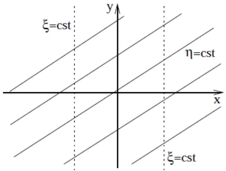
and the characteristics are the straight line graphs $3x-2y=c$. Hence we take $\eta =3x-2y$ and $\xi =x$.

(We can see that an $\eta$ and $\xi$ cross only once they are independent, i.e. $J\ne 0;\eta$ and $\xi$ have been properly chosen.)

This gives the solution

$$u(x,y)=e^{-4x}g(3x-2y)$$

where $g$ is a differentiable function defined over the real line. Simply specifying the solution at a given point (as in ODEs) does not uniquely determine $g$; we need to take a curve of initial conditions.

Suppose we specify values of $u(x,y)$ along a curve $\mathrm{\Gamma }$ in the plane. For example, let's choose $\mathrm{\Gamma }$ as the $x$-axis and gives values of $u(x,y)$ at points on $\mathrm{\Gamma }$, say

$$u(x,0)=\sin (x)$$

Then we need

$$u(x,0)=e^{-4x}g(3x)=\sin (x)\text{ i.e. }g(3x)=\sin (x)e^{4x}$$

and putting $t=3x$,

$$g(t)=\sin (t/3){\mathrm{e}}^{4t/3}$$

This determines $g$ and the solution satisfying the condition $u(x,0)=\sin (x)$ on $\mathrm{\Gamma }$ is

$$u(x,y)=\sin (x-2y/3)e^{-8y/3}$$

We have determined the unique solution of the PDE with $u$ specified along the $x$-axis. We do not have to choose an axis - say, along $x=y,u(x,y)=u(x,x)=x^4$. From the general solution this requires,

$$u(x,x)=e^{-4x}g(x)=x^4,\text{ so }g(x)=x^4{e}^{4x}$$

to give the unique solution

$$u(x,y)=(3x-2y{)}^4{e}^{8(x-y)}$$

satisfying $u(x,x)=x^4$.

However, not every curve in the plane can be used to determine $g$. Suppose we choose $\mathrm{\Gamma }$ to be the line $3x-2y=1$ and prescribe values of $u$ along this line, say

$$u(x,y)=u(x,(3x-1)/2)=x^2.$$

Now we must choose $g$ so that

$$e^{-4x}g(3x-(3x-1))=x^2.$$

This requires $g(1)=x^2{e}^{4x}$ (for all $x$ ). This is impossible and hence there is no solution taking the value $x^2$ at points $(x,y)$ on this line.

Last, we consider again $\mathrm{\Gamma }$ to be the line $3x-2y=1$ but choose values of $u$ along this line to be

$$u(x,y)=u(x,(3x-1)/2)=e^{-4x}.$$

Now we must choose $g$ so that

$$e^{-4x}g(3x-(3x-1))=e^{-4x}$$

This requires $g(1)=1$, condition satisfied by an infinite number of functions and hence there is an infinite number of solutions taking the values $e^{-4x}$ on the line $3x-2y=1$.

Depending on the initial conditions, the PDE has one unique solution, no solution at all or an infinite number or solutions. The difference is that the $x$-axis and the line $y=x$ are not the characteristics of the PDE while the line $3x-2y=1$ is a characteristic.

Example 2

$$x\frac{\partial u}{\partial x}-y\frac{\partial u}{\partial y}=u\text{ with }u=x^2\text{ on }y=x,1\le y\le 2$$

Characteristics:

$$\frac{\mathrm{d}y}{\mathrm{d}x}=-\frac{y}{x}\Rightarrow \mathrm{d}(xy)=0\Rightarrow xy=c,\text{ constant. }$$

So, take $\eta =xy$ and $\xi =x$. Then the equation becomes

$$xy\frac{\partial w}{\partial \eta }+x\frac{\partial w}{\partial \xi }-xy\frac{\partial w}{\partial \eta }=w\Rightarrow \xi \frac{\partial w}{\partial \xi }-w=0\Rightarrow \frac{\partial }{\partial \xi }\frac{w}{\xi }=0.$$

Finally the general solution is, $w=\xi g(\eta )$ or equivalently $u(x,y)=xg(xy)$. When $y=x$ with $1\le y\le 2,u=x^2$; so $x^2=xg\left(x^2\right)\Rightarrow g(x)=\sqrt{x}$ and the solution is

$$u(x,y)=x\sqrt{xy}.$$

This figure presents the characteristic curves given by $xy=$ constant. The red characteristics show the domain where the initial conditions permit us to determine the solution.

Application: Linear Waves

If $u$ is small (i.e. $u^2\ll u$ ), then the equation approximate to the linear wave equation

$$\frac{\partial u}{\partial t}+c\frac{\partial u}{\partial x}=0\text{ with }u(x,0)=f(x).$$

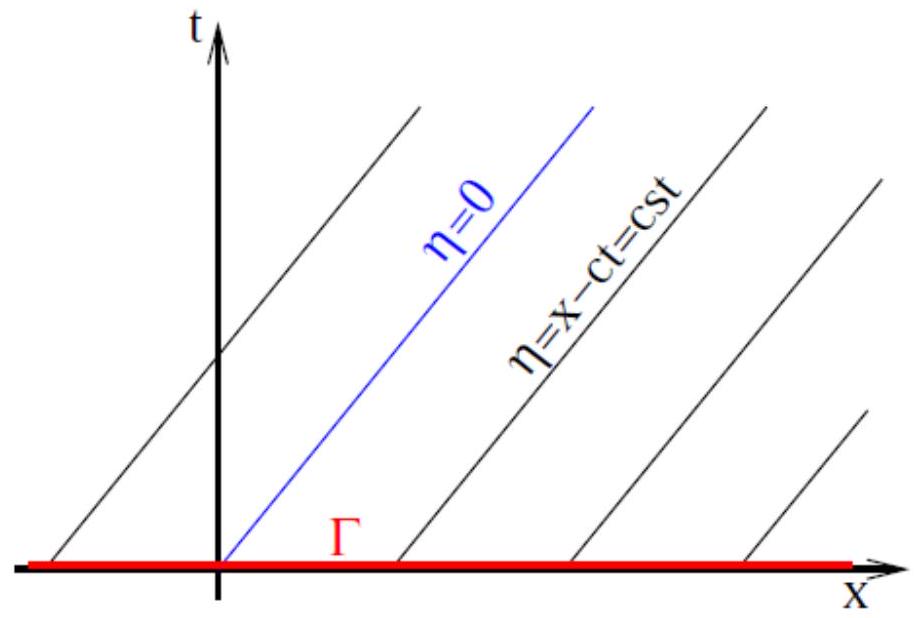
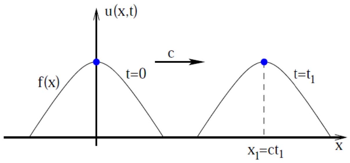
The solution of the equation of characteristics, $\mathrm{d}x/\mathrm{d}t=c$, gives the first integral of the PDE, $\eta (x,t)=x-ct$, and then general solution $u(x,t)=g(x-ct)$, where the function $g$ is determined by the initial conditions. Applying $u(x,0)=f(x)$ we find that the linear wave equation has the solution $u(x,t)=f(x-ct)$, which represents a wave (unchanging shape) propagating with constant wave speed $c$.

Note that $u$ is constant where $x-ct=$ constant, i.e. on the characteristics.

$2^{\text{nd}}$ order PDE solution

Second Order Linear PDE

Consider a general second order linear equation in two independent variables

$$a(x,y)\frac{{\partial }^{2}u}{\partial x^2}+2b(x,y)\frac{{\partial }^{2}u}{\partial x\partial y}+c(x,y)\frac{{\partial }^{2}u}{\partial y^2}+d(x,y)\frac{\partial u}{\partial x}+e(x,y)\frac{\partial u}{\partial y}+f(x,y)u=g(x,y);$$

Recall, for a first order linear and semilinear equation, $a\partial u/\partial x+b\partial u/\partial y=c$, we could define new independent variables, $\xi (x,y)$ and $\eta (x,y)$ with $J=\partial (\xi ,\eta )/\partial (x,y)\ne \{0,\mathrm{\infty }\}$, to reduce the equation to the simpler form, $\partial u/\partial \xi =\kappa (\xi ,\eta )$.

For the second order equation, can we also transform the variables from $(x,y)$ to $(\xi ,\eta )$ to put the equation into a simpler form?

As before we compute chain rule derivations

$$\begin{array}{c}\frac{\partial u}{\partial x}=\frac{\partial u}{\partial \xi }\frac{\partial \xi }{\partial x}+\frac{\partial u}{\partial \eta }\frac{\partial \eta }{\partial x},\frac{\partial u}{\partial y}=\frac{\partial u}{\partial \xi }\frac{\partial \xi }{\partial y}+\frac{\partial u}{\partial \eta }\frac{\partial \eta }{\partial y},\\ \frac{{\partial }^{2}u}{\partial x^2}=\frac{{\partial }^{2}u}{\partial {\xi }^2}{\left(\frac{\partial \xi }{\partial x}\right)}^2+2\frac{{\partial }^{2}u}{\partial \xi \partial \eta }\frac{\partial \xi }{\partial x}\frac{\partial \eta }{\partial x}+\frac{{\partial }^{2}u}{\partial {\eta }^2}{\left(\frac{\partial \eta }{\partial x}\right)}^2+\frac{\partial u}{\partial \xi }\frac{{\partial }^2\xi }{\partial x^2}+\frac{\partial u}{\partial \eta }\frac{{\partial }^2\eta }{\partial x^2},\\ \frac{{\partial }^{2}u}{\partial y^2}=\frac{{\partial }^{2}u}{\partial {\xi }^2}{\left(\frac{\partial \xi }{\partial y}\right)}^2+2\frac{{\partial }^{2}u}{\partial \xi \partial \eta }\frac{\partial \xi }{\partial y}\frac{\partial \eta }{\partial y}+\frac{{\partial }^{2}u}{\partial {\eta }^2}{\left(\frac{\partial \eta }{\partial y}\right)}^2+\frac{\partial u}{\partial \xi }\frac{{\partial }^2\xi }{\partial y^2}+\frac{\partial u}{\partial \eta }\frac{{\partial }^2\eta }{\partial y^2},\\ \frac{{\partial }^{2}u}{\partial x\partial y}=\frac{{\partial }^{2}u}{\partial {\xi }^2}\frac{\partial \xi }{\partial x}\frac{\partial \xi }{\partial y}+\frac{{\partial }^{2}u}{\partial \xi \partial \eta }(\frac{\partial \xi }{\partial x}\frac{\partial \eta }{\partial y}+\frac{\partial \xi }{\partial y}\frac{\partial \eta }{\partial x})+\frac{{\partial }^{2}u}{\partial {\eta }^2}\frac{\partial \eta }{\partial x}\frac{\partial \eta }{\partial y}+\frac{\partial u}{\partial \xi }\frac{{\partial }^2\xi }{\partial x\partial y}+\frac{\partial u}{\partial \eta }\frac{{\partial }^2\eta }{\partial x\partial y}.\end{array}$$

The equation becomes

$$\begin{array}{}\text{(3.1)}& A\frac{{\partial }^{2}u}{\partial {\xi }^2}+2B\frac{{\partial }^{2}u}{\partial \xi \partial \eta }+C\frac{{\partial }^{2}u}{\partial {\eta }^2}+F(u_{\xi },u_{\eta },u,\xi ,\eta )=0,\end{array}$$

where

$$\begin{array}{rl}A& =a{\left(\frac{\partial \xi }{\partial x}\right)}^2+2b\frac{\partial \xi }{\partial x}\frac{\partial \xi }{\partial y}+c{\left(\frac{\partial \xi }{\partial y}\right)}^2,\\ B& =a\frac{\partial \xi }{\partial x}\frac{\partial \eta }{\partial x}+b(\frac{\partial \xi }{\partial x}\frac{\partial \eta }{\partial y}+\frac{\partial \xi }{\partial y}\frac{\partial \eta }{\partial x})+c\frac{\partial \xi }{\partial y}\frac{\partial \eta }{\partial y},\\ C& =a{\left(\frac{\partial \eta }{\partial x}\right)}^2+2b\frac{\partial \eta }{\partial x}\frac{\partial \eta }{\partial y}+c{\left(\frac{\partial \eta }{\partial y}\right)}^2.\end{array}$$

Equation (3.1) can be simplified if we can choose $\xi$ and $\eta$ so that some of the coefficients $A$, $B$ or $C$ are zero. Let us define,

$$D_{\xi }=\frac{\partial \xi /\partial x}{\partial \xi /\partial y}\text{ and }{D}_{\eta }=\frac{\partial \eta /\partial x}{\partial \eta /\partial y}$$

then we can write

$$\begin{array}{rl}A& =(a{D}_{\xi }^2+2b{D}_{\xi }+c){\left(\frac{\partial \xi }{\partial y}\right)}^2\\ B& =(a{D}_{\xi }{D}_{\eta }+b(D_{\xi }+D_{\eta })+c)\frac{\partial \xi }{\partial y}\frac{\partial \eta }{\partial y}\\ C& =(a{D}_{\eta }^2+2b{D}_{\eta }+c){\left(\frac{\partial \eta }{\partial y}\right)}^2.\end{array}$$

Now consider the quadratic equation Vanish the item: $C\frac{{\partial }^{2}u}{\partial \eta 2}$ or $A\frac{{\partial }^{2}u}{\partial {\xi }^2}$

$$\begin{array}{}\text{(3.2)}& a{D}^2+2bD+c=0,\end{array}$$

whose solution is given by

$$D=\frac{-b\pm \sqrt{b^2-ac}}{a}.$$

• If the discriminant $b^2-ac\ne 0$:

equation (3.2) has two distinct roots; so, we can make both coefficients $A$ and $C$ zero if we arbitrarily take the root with the negative sign for $D_{\xi }$ and the one with the positive sign for $D_{\eta }$,

$$\begin{array}{}\text{(3.3)}& \begin{array}{rl}& D_{\xi }=\frac{\partial \xi /\partial x}{\partial \xi /\partial y}=\frac{-b-\sqrt{b^2-ac}}{a}\Rightarrow A=0,\\ & D_{\eta }=\frac{\partial \eta /\partial x}{\partial \eta /\partial y}=\frac{-b+\sqrt{b^2-ac}}{a}\Rightarrow C=0.\end{array}\end{array}$$

Then, using $D_{\xi }{D}_{\eta }=c/a$ and $D_{\xi }+D_{\eta }=-2b/a$ we have

$$B=\frac{2}{a}(ac-b^2)\frac{\partial \xi }{\partial y}\frac{\partial \eta }{\partial y}\Rightarrow B\ne 0.$$

Furthermore, if the discriminant $b^2-ac>0$:

then $D_{\xi }$ and $D_{\eta }$ as well as $\xi$ and $\eta$ are real. So, we can define two families of one-parameter characteristics of the PDE as the curves described by the equation $\xi (x,y)=$ constant and the equation $\eta (x,y)=$ constant. Differentiate $\xi$ along the characteristic curves given by $\xi =$ constant,

$$\mathrm{d}\xi =\frac{\partial \xi }{\partial x}\mathrm{d}x+\frac{\partial \xi }{\partial y}\mathrm{d}y=0$$

and make use of (3.3) to find that this characteristics satisfy

$$\begin{array}{}\text{(3.4)}& \frac{\mathrm{d}y}{\mathrm{d}x}=\frac{b+\sqrt{b^2-ac}}{a}.\end{array}$$

$$\frac{\partial \xi }{\partial x}\mathrm{d}x=-\frac{\partial \xi }{\partial y}\mathrm{d}y$$

Similarly we find that the characteristic curves described by $\eta (x,y)=$ constant satisfy

$$\begin{array}{}\text{(3.5)}& \frac{\mathrm{d}y}{\mathrm{d}x}=\frac{b-\sqrt{b^2-ac}}{a}.\end{array}$$

• If the discriminant $b^2-ac=0$:

equation (3.2) has one unique root and if we take this root for $D_{\xi }$ say, we can make the coefficient $A$ zero,

$$D_{\xi }=\frac{\partial \xi /\partial x}{\partial \xi /\partial y}=-\frac{b}{a}\Rightarrow A=0$$

To get $\eta$ independent of $\xi ,D_{\eta }$ has to be different from $D_{\xi }$, so $C\ne 0$ in this case, but $B$ is now given by

$$B=(-a\frac{b}{a}{D}_{\eta }+b(-\frac{b}{a}+D_{\eta })+c)\frac{\partial \xi }{\partial y}\frac{\partial \eta }{\partial y}=(-\frac{b^2}{a}+c)\frac{\partial \xi }{\partial y}\frac{\partial \eta }{\partial y},$$

so that $B=0$. When $b^2-ac=0$ the PDE has only one family of characteristic curves, for $\xi (x,y)=\mathrm{constant}$, whose equation is now

$$\begin{array}{}\text{(3.6)}& \frac{\mathrm{d}y}{\mathrm{d}x}=\frac{b}{a}.\end{array}$$

Classification of $2^{\text{nd }}$ Order Linear PDE

1. If $b^2>ac$ we can apply the change of variable $(x,y)\to (\eta ,\xi )$ to transform the original PDE to

$$\frac{{\partial }^{2}u}{\partial \xi \partial \eta }+(\text{ lower order terms })=0.$$

In this case the equation is said to be hyperbolic and has two families of characteristics given by equation (3.4) and equation (3.5).

2. If $b^2=ac$, a suitable choice for $\xi$ still simplifies the PDE, but now we can choose $\eta$ arbitrarily - provided $\eta$ and $\xi$ are independent - and the equation reduces to the form

$$\frac{{\partial }^{2}u}{\partial {\eta }^2}+(\text{ lower order terms })=0$$

The equation is said to be parabolic and has only one family of characteristics given by equation (3.6).

3. If $b^2<ac$ we can again apply the change of variables $(x,y)\to (\eta ,\xi )$ to simplify the equation but now this functions will be complex conjugate. To keep the transformation real, we apply a further change of variables $(\xi ,\eta )\to (\alpha ,\beta )$ via

$$\begin{array}{rl}& \alpha =\xi +\eta =2\mathrm{\Re }(\eta ),\\ & \beta =i(\xi -\eta )=2\mathrm{\Im }(\eta ),\end{array}$$$$\text{ i.e., }\frac{{\partial }^{2}u}{\partial \xi \partial \eta }=\frac{{\partial }^{2}u}{\partial {\alpha }^2}+\frac{{\partial }^{2}u}{\partial {\beta }^2}\text{ (via the chain rule); }$$

so, the equation can be reduced to

$$\frac{{\partial }^{2}u}{\partial {\alpha }^2}+\frac{{\partial }^{2}u}{\partial {\beta }^2}+(\text{ lower order terms })=0.$$

In this case the equation is said to be elliptic and has no real characteristics.

Example

• The wave equation,

$$\frac{{\partial }^{2}u}{\partial t^2}-c_w^2\frac{{\partial }^{2}u}{\partial x^2}=0,$$

is hyperbolic ( $b^2-ac=c_w^2>0$ ) and the two families of characteristics are described by $\mathrm{d}x/\mathrm{d}t=\pm c_w$ i.e. $\xi =x-c_{w}t$ and $\eta =x+c_{w}t$. So, the equation transforms into its canonical form ${\partial }^{2}u/\partial \xi \partial \eta =0$ whose solutions are waves travelling in opposite direction at speed $c_w$.

• The diffusion (heat conduction) equation,

$$\frac{{\partial }^{2}u}{\partial x^2}-\frac{1}{\kappa }\frac{\partial u}{\partial t}=0,$$

is parabolic ( $b^2-ac=0$ ). The characteristics are given by $\mathrm{d}t/\mathrm{d}x=0$ i.e. $\xi =t=$ constant.

• Laplace's equation,

$$\frac{{\partial }^{2}u}{\partial x^2}+\frac{{\partial }^{2}u}{\partial y^2}=0,$$

is elliptic $(b^2-ac=-1<0)$.

Example 1: Reduce to the canonical form

$$y^2\frac{{\partial }^{2}u}{\partial x^2}-2xy\frac{{\partial }^{2}u}{\partial x\partial y}+x^2\frac{{\partial }^{2}u}{\partial y^2}=\frac{1}{xy}(y^3\frac{\partial u}{\partial x}+x^3\frac{\partial u}{\partial y}).$$

Here $\begin{array}{l}a=y^2\\ b=-xy\\ c=x^2\end{array}\}$ so $b^2-ac=(xy{)}^2-x^2{y}^2=0\Rightarrow$ parabolic equation. On $\xi =$ constant,

$$\frac{\mathrm{d}y}{\mathrm{d}x}=\frac{b+\sqrt{b^2-ac}}{a}=\frac{b}{a}=-\frac{x}{y}\Rightarrow \xi =x^2+y^2.$$

We can choose $\eta$ arbitrarily provided $\xi$ and $\eta$ are independent. We choose $\eta =y$. (Exercise, try it with $\eta =x$.) Then

$$\begin{array}{rl}& \frac{\partial u}{\partial x}=2x\frac{\partial u}{\partial \xi },\frac{\partial u}{\partial y}=2y\frac{\partial u}{\partial \xi }+\frac{\partial u}{\partial \eta },\frac{{\partial }^{2}u}{\partial x^2}=2\frac{\partial u}{\partial \xi }+4x^2\frac{{\partial }^{2}u}{\partial {\xi }^2}\\ & \frac{{\partial }^{2}u}{\partial x\partial y}=4xy\frac{{\partial }^{2}u}{\partial {\xi }^2}+2x\frac{{\partial }^{2}u}{\partial \xi \partial \eta },\frac{{\partial }^{2}u}{\partial y^2}=2\frac{\partial u}{\partial \xi }+4y^2\frac{{\partial }^{2}u}{\partial {\xi }^2}+4y\frac{{\partial }^{2}u}{\partial \xi \partial \eta }+\frac{{\partial }^{2}u}{\partial {\eta }^2}\end{array}$$

and the equation becomes

$$\begin{array}{rl}& 2y^2\frac{\partial u}{\partial \xi }+4x^2{y}^2\frac{{\partial }^{2}u}{\partial {\xi }^2}-8x^2{y}^2\frac{{\partial }^{2}u}{\partial {\xi }^2}-4x^{2}y\frac{{\partial }^{2}u}{\partial \xi \partial \eta }+2x^2\frac{\partial u}{\partial \xi }+4x^2{y}^2\frac{{\partial }^{2}u}{\partial {\xi }^2}\\ +& 4x^{2}y\frac{{\partial }^{2}u}{\partial \xi \partial \eta }+x^2\frac{{\partial }^{2}u}{\partial {\eta }^2}=\frac{1}{xy}(2x{y}^3\frac{\partial u}{\partial \xi }+2x^{3}y\frac{\partial u}{\partial \xi }+x^3\frac{\partial u}{\partial \eta })\end{array}$$$$\text{i.e.}\frac{{\partial }^{2}u}{\partial {\eta }^2}-\frac{1}{\eta }\frac{\partial u}{\partial \eta }=0$$

This has solution

$$u=f(\xi )+{\eta }^{2}g(\xi ),$$

where $f$ and $g$ are arbitrary functions (via integrating factor method), i.e.

$$u=f(x^2+y^2)+y^{2}g(x^2+y^2).$$