
4. Kinodynamic Path Finding
Introduction
Kinodynamic : Kinematic + Dynamic:
The kinodynamic planning problem is to synthesize a robot motion subject to simultaneous kinematic constraints, such as avoiding obstacles, and dynamics constraints, such as modulus bounds on velocity, acceleration, and force. A kinodynamic solution is a mapping from time to generalized forces or accelerations. (From Kinodynamic Motion Planning)
- Differentially constrained
- Up to force (acceleration)
Reason: Straight-line connections between pairs of states are typically not valid trajectories due to the system’s differential constraints.
- Coarse-to-fine process
- Trajectory only optimizes locally
- Infeasible path means nothing to nonholonomic system
Examples:
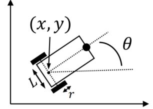
- Unicycle model:
Constraints:
- Differential drive model:
Constraints:
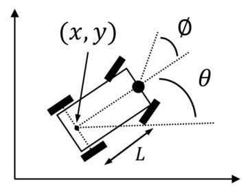
- Simplified car model:
Constraints:
State Lattice Planning
Basic idea
TODO: chap 2
- Recall the search-based path finding method in Chapter 2
- For planning, how to build a graph?
- Is this graph doable for our real robot?
Assume the robot, a mass point, is not satisfactory any more. We now require a graph with feasible motion connections. We manually create (build) a graph with all edges executable by the robot.
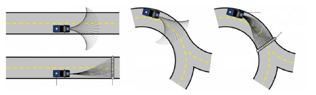
- Forward direction: discrete (sample) in control space
- Reverse direction: discrete (sample) in state space
This is the basic motivation for all kinodyanmic planning. State lattice planning is the most straight-forward one.
TODO: chap 2, 3
- In chapter 2, we discretize the control space (4 connections for 4-neighbor, 8 connections for 8-neighbor). We assume the robot can move in 4 / 8 directions.
- In chapter 3, we discretize the state space (position) and assume the robot can move in any direction.
For a robot model:
- Sample in control space: select a
, fix a time duration , forward simulate the system (numerical integration). - Forward simulation
- Fixed
- No mission guidance,
- East to implement
- Low planning efficiency
- Sample in state space: select a
, find the connection (a trajectory) between and - Backward calculation
- Need calculate
- Good mission guidance
- Hard to implement
- High planning efficiency
Sampling in control space
- State:
- Input:
- System equation:
where
Specially,
- Several-order integrator
nilpotent
The solution is:
where
If matrix
is nilpotent, i.e., , then has a closed-form expression in the form of an degree matrix polynomial in .
Note:
- During searching, the graph can be built when necessary.
- Create nodes (state) and edges (motion primitive) when nodes are newly discovered.
- Save computational time/space.
For every
- Pick a control vector
- Integrate the equation over short duration
- Add collision-free motions to the search tree
For simplified car model with state
- Select a
- Pick
- Integrate motion from
- Add result if collision-free
Sampling in state space
Build a lattice graph:
- Given an origin.
- for 8 neighbor nodes around the origin, feasible paths are found.
- extend outward to 24(=25-1) neighbors.
- complete lattice.
Comparison
Boundary Value Problem (BVP)
BVPis the basis of state sampled lattice planning.- No general solution. Case by case design.
- Often evolve complicated numerical optimization.
BVP: design a trajectory
With
Boundary conditions:
| Position | Velocity | Acceleration | |
|---|---|---|---|
Solve:
Optimal BVP (OBVP)[1]
Fix final state
Modelling:
- Objective: minimize the integral of squared jerk:
- State:
. Input: - System model:
/
Solving:
- By Pontryagin's Minimum Principle, we first introduce the costate:
- Define the Hamiltonian function:
Generally:
where
is the final state and is the transition cost. Write the Hamiltonian and costate:
Suppose the optimal input is
and the optimal state is , then the necessary conditions for optimality are: with the boundary condition of:
and the optimal input
satisfies:
The costate is solved as:
(For later convenience)
The optimal input is solved as:
The optimal state trajectory is solved as:
with initial state:
The remaining unknowns
Solving for the unknown coefficients yields
where
And the cost is:
- Similar solution can also be found when
is partially defined - Same solving process holds for
The boundary condition:
- For fixed final state problem:
Not differentiable. So we discard this condition, and use given
- For (partially)-free final state problem:
We have boundary condition for other costate:
Free v & a (Homework)
The Hamiltonian function is shown in the last section:
By utilizing Pontryagin's Minimum Principle, we have (Also shown in the last section):
With boundary condition for
Thus, we have:
and
The optimal input is solved as:
By integrating the optimal input, we have the optimal state trajectory as:
With known
Thus:
It shows that
Thus, the optimal
And
TBC
Mueller M W, Hehn M, D'Andrea R. A computationally efficient motion primitive for quadrocopter trajectory generation[J]. IEEE transactions on robotics, 2015, 31(6): 1294-1310. ↩︎