Angle

Introduction [1]

Unfortunately, similar to the displacement-based approach, a bearing-constrained formation requires either the global coordinate system for each agent or developing observers based on inter-agent communications. The authors in some research achieved bearing-based formation control in the absence of the global coordinate system, but each agent should have a controllable quantity determining the relationship between the local body frame and the global coordinate frame.

2D Angle Rigidity [1][3]

Definition of angle rigidity in 2D

We still use ${\mathit{z}}_{ij}={\mathit{p}}_i-{\mathit{p}}_j,{\mathit{g}}_{ij}=\frac{{\mathit{p}}_i-{\mathit{p}}_j}{\parallel {\mathit{p}}_i-{\mathit{p}}_j\parallel }$ from the Chapter: Bearing Rigidity in arbitary dimension

In this section, we develop an angle rigidity theory to investigate how to encode geometric shapes of graphs embedded in the plane through angles only.

For a framework $(\mathcal{G},\mathit{p})$ in ${\mathbb{R}}^2$, we will employ ${\mathit{g}}_{ij}^{\mathrm{\top }}{\mathit{g}}_{ik}$ as the object we will constrain, which is actually the cosine of the angle between edges ${\mathit{z}}_{ij}$ and ${\mathit{z}}_{ik}$. Let ${\mathcal{T}}_{\mathcal{G}}=\{(i,j,k)\in {\mathcal{V}}^3:(i,j),(i,k)\in \mathcal{E},j<k\}$, then $\{{\mathit{g}}_{ij}^{\mathrm{\top }}{\mathit{g}}_{ik}=c_{ijk}:c_{ijk}\in [-1,1],(i,j,k)\in {\mathcal{T}}_{\mathcal{G}}\}$ is the set of constraints on all angles in $(\mathcal{G},\mathit{p})$.

We can also use $\mathcal{A}\subset \mathcal{V}\times \mathcal{V}\times \mathcal{V}$ to denote the angle set, each element of which is an ordered triplet. Denote $|\mathcal{A}|=M$. Then, the combination of the vertex set $\mathcal{V}$, the angle set $\mathcal{A}$, and the position vector \boldsymbol{p}_ is called an angularity, which we denote by $\mathbb{A}(\mathcal{V},\mathcal{A},\mathit{p})$.

For the angle, given nonoverlapping positions ${\mathit{p}}_i$, ${\mathit{p}}_j$, and ${\mathit{p}}_k$, the angle $\measuredangle ijk\in [0,2\pi )$ can be uniquely calculated from

$$\measuredangle ijk=\{\begin{array}{ll}\arccos ({\mathit{g}}_{ij}^{\mathrm{\top }}{\mathit{g}}_{kj})& \text{if }{\mathit{g}}_{ij}^{\perp }\cdot {\mathit{g}}_{kj}⩾0\\ 2\pi -\arccos ({\mathit{g}}_{ij}^{\mathrm{\top }}{\mathit{g}}_{kj})& \text{otherwise}\end{array}.$$

where $\measuredangle ijk$ for each triplet $(i,j,k)$ is measured counter-clockwise in the range $[0,2\pi )$ where the ray starts by crossing the vertex $i$, rotating around the vertex $j$, and finally cross the vertex $k$. ${\mathit{g}}_{ij}^{\perp }=Q_0{\mathit{g}}_{ij}=\left[\begin{array}{cc}0& -1\\ 1& 0\end{array}\right]{\mathit{g}}_{ij}$ is the vector obtained by rotating ${\mathit{g}}_{ij}$ counterclockwise by $\pi /2$.

We should note that a framework often has redundant angle information for shape determination.

Figure 1: (a) A globally and infinitesimally angle rigid framework; (b) A framework that is not angle rigid. (c) A globally and infinitesimally angle rigid framework; (d) A globally angle rigid framework.

For example, in Figure 1(a), once ${\mathit{g}}_{12}^{\mathrm{\top }}{\mathit{g}}_{13}$ and ${\mathit{g}}_{21}^{\mathrm{\top }}{\mathit{g}}_{23}$ are available, it holds that ${\mathit{g}}_{31}^{\mathrm{\top }}{\mathit{g}}_{32}=\cos (\pi -\arccos ({\mathit{g}}_{12}^{\mathrm{\top }}{\mathit{g}}_{13})-\arccos ({\mathit{g}}_{21}^{\mathrm{\top }}{\mathit{g}}_{23}))$. That is, the information of partial angles in the graph is often sufficient to recognize a framework. Therefore, by employing a subset ${\mathcal{T}}_{\mathcal{G}}^{\ast }\subset {\mathcal{T}}_{\mathcal{G}}$ with $|{\mathcal{T}}_{\mathcal{G}}^{\ast }|=w$, we will try to study whether $(\mathcal{G},\mathit{p})$ can be uniquely determined by $\{{\mathit{g}}_{ij}^{\mathrm{\top }}{\mathit{g}}_{ik}\in [-1,1]:(i,j,k)\in {\mathcal{T}}_{\mathcal{G}}^{\ast }\}$ based on the angle rigidity theory to be developed in this paper. Note that although ${\mathcal{T}}_{\mathcal{G}}^{\ast }$ is only a subset of ${\mathcal{T}}_{\mathcal{G}}$, the elements in ${\mathcal{T}}_{\mathcal{G}}^{\ast }$ should involve all vertices in $\mathcal{G}$, otherwise the shape of $(\mathcal{G},\mathit{p})$ can never be determined. Moreover, we call ${\mathcal{T}}_{\mathcal{G}}^{\ast }$ the angle index set.

For a framework $(\mathcal{G},\mathit{p})$, the angle rigidity function corresponding to a given angle index set ${\mathcal{T}}_{\mathcal{G}}^{\ast }$ can be written as

$${\mathit{a}}_{{\mathcal{T}}_{\mathcal{G}}^{\ast }}(\mathit{p})=(\cdots ,{\mathit{g}}_{ij}^{\mathrm{\top }}(\mathit{p}){\mathit{g}}_{ik}(\mathit{p}),\cdots {)}^{\mathrm{\top }},(i,j,k)\in {\mathcal{T}}_{\mathcal{G}}^{\ast }.$$

For the sake of notational simplicity, we denote ${\mathit{a}}_{\mathcal{G}}(\mathit{p})={\mathit{a}}_{{\mathcal{T}}_{\mathcal{G}}}(\mathit{p})$.

It is easy to see that whether ${\mathit{a}}_{{\mathcal{T}}_{\mathcal{G}}^{\ast }}(\mathit{p})$ can determine a unique shape congruent to $\mathit{p}$ is determined by the choice of ${\mathcal{T}}_{\mathcal{G}}^{\ast }$. As a result, the definitions of angle rigidity must be associated with ${\mathcal{T}}_{\mathcal{G}}^{\ast }$. We present the following definitions.

Definition: Equivalency and congruency abut angle rigidity

Two angularities $\mathbb{A}(\mathcal{V},\mathcal{A},\mathit{p})$ and ${\mathbb{A}}^{\prime }(\mathcal{V},\mathcal{A},{\mathit{p}}^{\prime })$ with the same $\mathcal{V}$ and $\mathcal{A}$ are equivalent if

$$\measuredangle ijk({\mathit{p}}_i,{\mathit{p}}_j,{\mathit{p}}_k)=\measuredangle ijk({\mathit{p}}_i^{\prime },{\mathit{p}}_j^{\prime },{\mathit{p}}_k^{\prime }),\mathrm{\forall }(i,j,k)\in \mathcal{A}.$$

They are congruency if

$$\measuredangle ijk({\mathit{p}}_i,{\mathit{p}}_j,{\mathit{p}}_k)=\measuredangle ijk({\mathit{p}}_i^{\prime },{\mathit{p}}_j^{\prime },{\mathit{p}}_k^{\prime }),\mathrm{\forall }i,j,k\in \mathcal{V}.$$

Definition: angle rigid

A framework $(\mathcal{G},\mathit{p})$ is angle rigid if there exist an angle index set ${\mathcal{T}}_{\mathcal{G}}^{\ast }$ and a neighborhood ${\mathcal{U}}_p$ of $\mathit{p}$ such that ${\mathit{a}}_{{\mathcal{T}}_{\mathcal{G}}^{\ast }}^{-1}({\mathit{a}}_{{\mathcal{T}}_{\mathcal{G}}^{\ast }}(\mathit{p}))\cap {\mathcal{U}}_p={\mathit{a}}_{\mathcal{K}}^{-1}({\mathit{a}}_{\mathcal{K}}(\mathit{p}))\cap {\mathcal{U}}_p$.

With equivalent and congruent relationships, here is another type of definition: An angularity $\mathbb{A}(\mathcal{V},\mathcal{A},\mathit{p})$ is angle rigid if there exists an $\epsilon >0$ such that every angularity ${\mathbb{A}}^{\prime }(\mathcal{V},\mathcal{A},{\mathit{p}}^{\prime })$ that is equivalent to it and satisfies $\parallel {\mathit{p}}^{\prime }-\mathit{p}\parallel <\epsilon$ is congruent to it.

Definition of angle rigidity with equivalent and congruent implies that every configuration which is sufficiently close to $\mathit{p}$ and satisfies all the angle constraints formed by $\mathcal{A}$ has the same magnitudes of the angles formed by any three vertices in $\mathcal{V}$ as the original configuration at $\mathit{p}$.

Definition: globally angle rigid

A framework $(\mathcal{G},\mathit{p})$ is globally angle rigid if there exists an angle index set ${\mathcal{T}}_{\mathcal{G}}^{\ast }$ such that ${\mathit{a}}_{{\mathcal{T}}_{\mathcal{G}}^{\ast }}^{-1}({\mathit{a}}_{{\mathcal{T}}_{\mathcal{G}}^{\ast }}(\mathit{p}))={\mathit{a}}_{\mathcal{K}}^{-1}({\mathit{a}}_{\mathcal{K}}(\mathit{p}))$.

With equivalent and congruent relationships, here is another type of definition: An angularity $\mathbb{A}(\mathcal{V},\mathcal{A},\mathit{p})$ is globally angle rigid if every angularity that is equivalent to it is also congruent to it.

Definition: minimally angle rigid

A framework $(\mathcal{G},\mathit{p})$ is minimally angle rigid if $(\mathcal{G},\mathit{p})$ is angle rigid, and deletion of any edge will make $(\mathcal{G},\mathit{p})$ not angle rigid.

By these definitions, the frameworks (a) and (c) in Figure 1 are both globally angle rigid. For the framework (b), by moving the vertices along the blue arrows, $f_{\mathcal{G}}$ is invariant but the shape is deformed, thus (b) is not angle rigid. For the framework (d), since the graph is complete, it obviously holds ${\mathit{a}}_{\mathcal{G}}^{-1}({\mathit{a}}_{\mathcal{G}}(\mathit{p}))={\mathit{a}}_{\mathcal{K}}^{-1}({\mathit{a}}_{\mathcal{K}}(\mathit{p}))$, thus (d) is globally angle rigid. Note that the shape of (d) still cannot be determined by angles uniquely.

As is clear from Definitions of angle rigidity and global angle rigidity, global angle rigidity always implies angle rigidity. A natural question to ask is whether angle rigidity also implies global angle rigidity. In fact, for bearing rigidity, it has been shown that indeed global bearing rigidity and bearing rigidity are equivalent. However, this is not the case for angle rigidity:

Theorem 0: Nonequivalence between angle rigidity and global angle rigidity

An angle rigid angularity $\mathbb{A}(\mathcal{V},\mathcal{A},\mathit{p})$ is not necessarily globally angle rigid.

Figure 2: Flex ambiguity in angle rigid angularity.

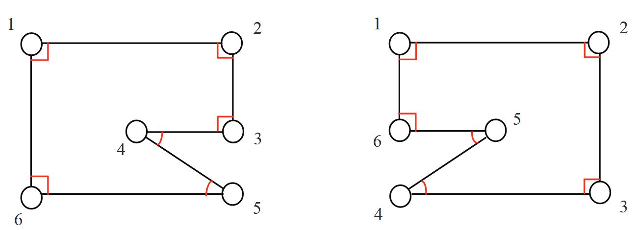
Here is an example, see Figure 2. $\mathbb{A}(\mathcal{V},\mathcal{A},\mathit{p})$ is angle rigid, but not globally angle rigid.

• Since two of its angles $\measuredangle 321$ and $\measuredangle 132$ have been constrained, the remaining $\measuredangle 213$ is uniquely determined to be $\pi -\measuredangle 321-\measuredangle 132$, no matter how $\mathit{p}$ is locally perturbed.
• The constraint on $\measuredangle 234$ requires $4$ must lie in the ray starting from $3$ and rotating from ray $32$ counter-clockwise by ${30}^{\circ }$; at the same time, the constraint on $\measuredangle 142$ requires $4$ must lie on the arc passing through $1$ and $2$ such that the inscribed angle $\measuredangle 142$ is ${45}^{\circ }$. No matter how $\mathit{p}$ is locally perturbed, there is only one unique position for $4$ in the neighborhood of its current given coordinates because the two intersection points between the ray and the arc are not in the same local neighborhood. This local uniqueness implies that this four-vertex angularity is angle rigid (when $4$’s position is uniquely determined, any angle associated with it is also uniquely determined).
• Note that there is the other intersection point $4^{\prime }$ as shown in Figure 2 satisfying the angle constraints given in $\mathcal{A}$.

Bearing rigidity is a global property because the bearing constraints always represent linear constraints in the end point’s position and two noncollinear rays have at most one intersection.

In contrast, the angle constraint can be:

• linear constraint in $\mathit{p}$ when it requires the corresponding vertex to be on a ray;
• quadratic in $\mathit{p}$ when it restricts the corresponding vertex to be on an arc passing through other vertices.

The possible nonlinearity in the angle constraints gives rise to potential ambiguity of the vertices’ positions under the given angle constraints.

Figure 3: Nongeneric p changes rigidity. (a) Not rigid; (b) Angle rigid; (c) Globally angle rigid.

Note that the embedding of $\mathit{p}$ in the plane may affect the rigidity of $\mathbb{A}$. Consider the $3$-vertex angularity as embedded in three different situations in Figure 3 when its angle set $\mathcal{A}$ contains only one element $(2,1,3)$.

• Figure 3(a) shows that $1$, $2$, and $3$ are not collinear, and then this angularity is in general not rigid since if we perturb point $1$ in an arc with $2$ and $3$ as the arc’s ending points, $\measuredangle 213$ can be the same while angles $\measuredangle 123$ and $\measuredangle 132$ change.
• In Figure 3(b), $1$, $2$, and $3$ are collinear and $1$ is on one side; in this case, if the angle constraint happens to be $\measuredangle 213=0$, then one can check the angularity becomes angle rigid, although it is not globally rigid since the angle of $\measuredangle 132$ changes by $180$ degree if we swap $2$ and $3$.
• In Figure 3(c), $1$, $2$, and $3$ are collinear and $1$ is in the middle; when the constraint becomes $\measuredangle 213=\pi$, one can check that the angularity is not only rigid, but also globally rigid (swapping of $2$ and $3$ in this case does not change the resulting angles $\measuredangle 132$, $\measuredangle 123$ being zero).

So the angularity $\mathbb{A}(\{1,2,3\},\{(2,1,3)\},\mathit{p})$ is generically not rigid, but rarely rigid depending on $\mathit{p}$. To clearly describe this relationship between angle rigidity and $\mathit{p}$, like in standard rigidity theory, we define what we mean by generic positions.

::: warnig Definition: Generic position The position vector $\mathit{p}$ is said to be generic if its components are algebraically independent. Then, we say an angularity is generically (respectively globally) angle rigid if its $\mathit{p}$ is generic and it is (respectively globally) angle rigid. :::

An example for nongeneric positions is the case when three points are collinearly positioned. Note that angle rigidity for $\mathbb{A}(\mathcal{V},\mathcal{A},\mathit{p})$ with generic $\mathit{p}$ represents the common property of the combination $(\mathcal{V},\mathcal{A})$ from a topological perspective, which is also referred to as generic angle rigidity. For convenience, we also say an angularity is generic if its $\mathit{p}$ is generic. Now we provide some sufficient conditions for an angularity to be globally angle rigid. Towards this end, we need to introduce some concepts and operations.

Definition: subangularity

For two angularities $\mathbb{A}(\mathcal{V},\mathcal{A},\mathit{p})$ and ${\mathbb{A}}^{\prime }({\mathcal{V}}^{\prime },{\mathcal{A}}^{\prime },{\mathit{p}}^{\prime })$, we say $\mathbb{A}$ is a subangularity of ${\mathbb{A}}^{\prime }$ if $\mathcal{V}\subset {\mathcal{V}}^{\prime },\mathcal{A}\subset {\mathcal{A}}^{\prime }$ and $\mathit{p}$ is the corresponding subvector of ${\mathit{p}}^{\prime }$.

We first clarify that for the smallest angularities, namely those that contain only three vertices, there is no gap between angle rigidity and global angle rigidity assuming generic positions.

Lemma 0

For a 3-vertex angularity, if it is generically angle rigid, it is also generically globally angle rigid.

Proof: For this 3-vertex angularity $\mathbb{A}(\mathcal{V},\mathcal{A},\mathit{p})$, since it is angle rigid and $\mathit{p}$ is generic, $\mathcal{A}$ must contain at least two elements, or said differently, two of the interior angles of the triangle formed by the three vertices are constrained. Again since $\mathit{p}$ is generic, the sum of the three interior angles in this triangle has to be $\pi$, and thus the magnitude of this triangle’s remaining interior angle is uniquely determined too. Therefore, $\mathbb{A}$ is generically globally angle rigid.

$◻$

Now, we define linear and quadratic constraints.

Definition: Linear and quadratic constraints

• For a given angularity $\mathbb{A}(\mathcal{V},\mathcal{A},\mathit{p})$, a new vertex $i$ positioned at ${\mathit{p}}_i$ is linearly constrained w.r.t. $\mathbb{A}$ if there is $j\in \mathcal{V}$ such that ${\mathit{p}}_i\ne {\mathit{p}}_j$ and ${\mathit{p}}_i$ is constrained to be on a ray starting from ${\mathit{p}}_j$;
• $i$ is quadratically constrained w.r.t. $\mathbb{A}$ if there are $j,k\in \mathcal{V}$ such that $\{{\mathit{p}}_i,{\mathit{p}}_j,{\mathit{p}}_k\}$ is generic and ${\mathit{p}}_i$ is constrained to be on an arc with ${\mathit{p}}_j$ and ${\mathit{p}}_k$ being the arc’s two ending points.

Correspondingly, we call $i$’s constraint in the former case a linear constraint and in the latter case a quadratic constraint w.r.t. $\mathbb{A}$.

As shown in Figure 2, $\measuredangle 234={30}^{\circ }$ is a linear constraint for the end vertex $4$ since ${\mathit{p}}_4$ is constrained to be on a ray starting from ${\mathit{p}}_3$, while $\measuredangle 142={45}^{\circ }$ is a quadratic constraint for $4$ because ${\mathit{p}}_4$ is constrained to be on the major arc $\stackrel{⌢}{12}$.

Similar to Henneberg’s construction in distance rigidity, in the following, we define two types of vertex addition operations in angle rigidity to demonstrate how a bigger angularity might grow from a smaller one, which are shown in Figure 4.

Figure 4: Type-I vertex addition and Type-II vertex addition. (a) Case 1 in Type-I vertex addition. (b) Case 2 in Type-I vertex addition. (c) Case 3 in Type-I vertex addition. (d) Case 1 in Type-II vertex addition. (e) Case 2 in Type-II vertex addition.

Definition: Type-I vertex addition

For a given angularity $\mathbb{A}(\mathcal{V},\mathcal{A},\mathit{p})$, we say the angularity ${\mathbb{A}}^{\prime }$ with the augmented vertex set $\{\mathcal{V}\cup \{i\}\}$ is obtained from $\mathbb{A}$ through a Type-I vertex addition if the new vertex $i$’s constraints w.r.t. $\mathbb{A}$ contain at least one of the following.

• Case 1: 2 linear constraints, not aligned, associated with 2 distinct vertices in $\mathcal{V}$ (1 vertex for 1 constraint and the other vertex for the other constraint).
• Case 2: 1 linear constraint and 1 quadratic constraint associated with 2 distinct vertices in $\mathcal{V}$ (1 for the former and both for the latter).
• Case 3: 2 different quadratic constraints associated with 3 vertices in $\mathcal{V}$ (2 for each and 1 is shared by both), and the positions of $i$ and these 3 vertices are generic.

Definition: Type-II vertex addition

For a given angularity $\mathbb{A}(\mathcal{V},\mathcal{A},\mathit{p})$, we say the angularity ${\mathbb{A}}^{\prime }$ with the augmented vertex set $\{\mathcal{V}\cup \{i\}\}$ is obtained from $\mathbb{A}$ through a Type-II vertex addition if the new vertex $i$’s constraints w.r.t. $\mathbb{A}$ contain at least one of the following:

• Case 1: 1 linear constraint and 1 quadratic constraint associated with three distinct vertices in $\mathcal{V}$ (1 for the former and the other 2 for the latter);
• Case 2: 2 different quadratic constraints associated with 4 vertices in $\mathcal{V}$ (2 for the former and the other 2 for the latter), and the positions of $i$ and these 4 vertices are generic.

Remark:

1. Although the types of constraints are similar between Case 2 of Type-I and Case 1 of Type-II, the numbers of vertices involved in Case 2 of Type-I and Case 1 of Type-II differ in these two types of vertex addition operations. Similarly, those in Case 3 of Type-I and Case 2 of Type-II are also different.
2. Note that in these two vertex addition operations, the involved vertices are required to be in generic positions. However, the overall angle rigid angularity ${\mathbb{A}}^{\prime }$ constructed through a sequence of vertex addition operations is not necessarily generic, and an example is given in Figure 5.

Figure 5: Overall angularity is not necessarily generic. (a) Point 4 is unique when {1,3,4} are generic. (b) Point 4 is not unique when {1,3,4} are not generic. (c) {2,3,5} are not generic but angularity is rigid.

Now we are ready to present a sufficient condition for global angle rigidity using Type-I vertex addition.

Proposition 1: Sufficient condition for global angle rigidity

An angularity is globally angle rigid if it can be obtained through a sequence of Type-I vertex additions from a generically angle rigid $3$-vertex angularity.

Details of Proof

According to Lemma 0, the generically angle rigid $3$-vertex angularity is globally angle rigid. Consider the three conditions in the Type-I vertex addition.

• If case 1 applies, then the position ${\mathit{p}}_i$ of the newly added vertex $i$ is unique since two rays, not aligned, starting from two different points may intersect only at one point;
• If case 2 applies, ${\mathit{p}}_i$ is again unique since a ray starting from the end point of an arc may intersect with the arc at most at one other point;
• If case 3 applies, ${\mathit{p}}_i$ is unique since two arc sharing one end point on different circles can only intersect at most at one other point.

Therefore, ${\mathit{p}}_i$ is always globally uniquely determined. After ${\mathit{p}}_i$ is globally uniquely determined, all the angles associated with ${\mathit{p}}_i$ are also globally uniquely determined. Because each Type-I vertex addition operation can guarantee a unique adding point ${\mathit{p}}_i$, we conclude that the obtained angularity after a sequence of Type-I vertex additions is globally angle rigid.

$◻$

In comparison, Type-II vertex additions can only guarantee angle rigidity, but not global angle rigidity.

Proposition 2: Sufficient condition for angle rigidity

An angularity is angle rigid if it can be obtained through a sequence of Type-II vertex additions from a generically angle rigid $3$-vertex angularity.

The proof can be easily constructed following similar arguments as those for Proposition 1. The only difference is that ${\mathit{p}}_i$ now may have two solutions and is only unique locally.

After having presented our results on angularity and angle rigidity, in the following section, we discuss infinitesimal angle rigidity, which relates closely to infinitesimal motion.

Infinitesimal Angle Rigidity

From [1]

Similar to distance and bearing rigidity theory, we define the infinitesimal angle motion as a motion preserving the invariance of ${\mathit{a}}_{{\mathcal{T}}_{\mathcal{G}}^{\ast }}(\mathit{p})$. The velocity $\mathit{v}=\dot{\mathit{p}}$ corresponding to an infinitesimal motion should satisfy ${\dot{\mathit{a}}}_{{\mathcal{T}}_{\mathcal{G}}^{\ast }}(\mathit{p})=0$, which is equivalent to the following equation

$$\begin{array}{}\text{(1)}& {\dot{\mathit{g}}}_{ij}^{\mathrm{\top }}{\mathit{g}}_{ik}+{\mathit{g}}_{ij}^{\mathrm{\top }}{\dot{\mathit{g}}}_{ik}=0,(i,j,k)\in {\mathcal{T}}_{\mathcal{G}}^{\ast }.\end{array}$$

From the Chapter: Lemma 6 of Chapter: Bearing rigidity, we know that $\frac{\partial {\mathit{g}}_{ij}}{\partial {\mathit{z}}_{ij}}=\frac{1}{\parallel {\mathit{z}}_{ij}\parallel }{P}_{ij}$, where $P_{ij}\triangleq P({\mathit{g}}_{ij})$, $P(\cdot ):{\mathbb{R}}^2\to {\mathbb{R}}^{2\times 2}$ is a projection matrix defined as $P(x)=I_2-\mathit{x}{\mathit{x}}^{\mathrm{\top }}$, $\mathit{x}\in {\mathbb{R}}^2$ is a unit vector. Then we have ${\dot{\mathit{g}}}_{ij}=\frac{1}{\parallel {\mathit{z}}_{ij}\parallel }{P}_{ij}{\dot{\mathit{z}}}_{ij}$. Let ${\mathit{b}}_{\mathcal{G}}(\mathit{p})=(\cdots ,{\mathit{g}}_{ij}^{\mathrm{\top }}(\mathit{p}),\cdots {)}^{\mathrm{\top }}$, where $(i,j)\in \mathcal{E}$, and $R_g\triangleq \frac{\partial {\mathit{a}}_{{\mathcal{T}}_{\mathcal{G}}^{\ast }}}{\partial \mathit{g}}$. It follows from the chain rule that

$${\dot{\mathit{a}}}_{{\mathcal{T}}_{\mathcal{G}}^{\ast }}=\frac{\partial {\mathit{a}}_{{\mathcal{T}}_{\mathcal{G}}^{\ast }}}{\partial {\mathit{b}}_{\mathcal{G}}}\frac{\partial {\mathit{b}}_{\mathcal{G}}}{\partial \mathit{z}}\frac{\partial \mathit{z}}{\partial \mathit{p}}\dot{\mathit{p}}=R_g(\mathit{p})\mathrm{diag}(\frac{P_{ij}}{\parallel {\mathit{z}}_{ij}\parallel })\overline{H}\dot{\mathit{p}}=R_{{\mathcal{T}}_{\mathcal{G}}^{\ast }}(\mathit{p})\dot{\mathit{p}},$$

where $\overline{H}=H\otimes I_2$, $R_{{\mathcal{T}}_{\mathcal{G}}^{\ast }}(\mathit{p})\triangleq R_g(\mathit{p})\mathrm{diag}(\frac{P_{ij}}{\parallel {\mathit{z}}_{ij}\parallel })\overline{H}=R_g(\mathit{p})R_B(\mathit{p})\in {\mathbb{R}}^{w\times 2n}$ is termed the angle rigidity matrix, $R_{\mathcal{B}}=\frac{\partial g(\mathit{p})}{\partial \mathit{p}}$ is actually the bearing rigidity matrix. Therefore, equation $(1)$ is equivalent to $R_{{\mathcal{T}}_{\mathcal{G}}^{\ast }}(\mathit{p})\dot{\mathit{p}}=\mathbf{0}$.

Next we define infinitesimal angle rigidity, to do this, we should distinguish all trivial motions for an angle-constrained geometric shape. By an intuitive observation, the motions always preserving invariance of angles in the framework are translations, rotations, and scalings. Therefore, the dimension of the trivial motion space is $2+1+1=4$. Note that the trivial motion space is always a subspace of $\mathrm{Null}(R_{{\mathcal{T}}_{\mathcal{G}}^{\ast }})$, implying that $\dim (\mathrm{Null}(R_{{\mathcal{T}}_{\mathcal{G}}^{\ast }}))\ge 4$. We present the following definition.

Definition: infinitesimally angle rigid

A framework $(\mathcal{G},\mathit{p})$ is infinitesimally angle rigid if there exists an angle index set ${\mathcal{T}}_{\mathcal{G}}^{\ast }$ such that every possible motion satisfying equation $(1)$ is trivial, or equivalently, $\dim (\mathrm{Null}(R_{{\mathcal{T}}_{\mathcal{G}}^{\ast }}))=4$.

By this definition, the frameworks in Figure 1 (a) and (c) are both infinitesimally angle rigid. The frameworks (b) and (d) are not infinitesimally angle rigid since they both have nontrivial infinitesimal angle motions, which are interpreted by the arrows in blue.

In this paper, we say an angle index set ${\mathcal{T}}_{\mathcal{G}}^{\ast }$ supports or is suitable for (global, minimal, infinitesimal) angle rigidity of $(\mathcal{G},\mathit{p})$ if ${\mathcal{T}}_{\mathcal{G}}^{\ast }$ makes the condition in the corresponding definition valid. We say ${\mathcal{T}}_{\mathcal{G}}^{\ast }$ is minimally suitable if ${\mathcal{T}}_{\mathcal{G}}^{\ast }$ is suitable and no proper subset of ${\mathcal{T}}_{\mathcal{G}}^{\ast }$ can be suitable.

It is easy to see from Definitions above that the angle rigidity property of a framework $(\mathcal{G},\mathit{p})$ is completely dependent on $\mathcal{G}$ and $\mathit{p}$. After $(\mathcal{G},\mathit{p})$ is given, whether a suitable ${\mathcal{T}}_{\mathcal{G}}^{\ast }$ exists becomes certain. However, even for an angle rigid framework, there may exist ${\mathcal{T}}_{\mathcal{G}}^{\ast }$ such that the conditions in the angle rigidity definitions are invalid. For example, if we choose ${\mathcal{T}}_{\mathcal{G}}^{\ast }={\mathcal{T}}_T$ where $T$ is a spanning tree of $\mathcal{G}$, ${\mathcal{T}}_{\mathcal{G}}^{\ast }$ can never support angle rigidity of $(\mathcal{G},\mathit{p})$. On the other hand, there may exist multiple choices of ${\mathcal{T}}_{\mathcal{G}}^{\ast }$ supporting angle rigidity of a rigid framework. In Subsection, Algorithm 1 will be given to construct a suitable angle index set.

From [3]

Angle Rigidity Matrix

We consider an arbitrary element $(i,j,k)$ in A and denote the corresponding angle constraint by $\measuredangle ijk({\mathit{p}}_i,{\mathit{p}}_j,{\mathit{p}}_k)=\beta \in [0,2\pi )$, or in shorthand $\measuredangle ijk=\beta$. From the definition of the dot product, one has

$$\cos \beta =\frac{({\mathit{p}}_i-{\mathit{p}}_j{)}^{\mathrm{\top }}}{\parallel {\mathit{p}}_i-{\mathit{p}}_j\parallel }\frac{({\mathit{p}}_k-{\mathit{p}}_j{)}^{\mathrm{\top }}}{\parallel {\mathit{p}}_k-{\mathit{p}}_j\parallel }={\mathit{g}}_{ij}^{\mathrm{\top }}{\mathit{g}}_{kj}$$

Differentiating both sides of formula above w.r.t. time leads to

$$\begin{array}{rl}(-\sin \beta )\dot{\beta }& ={\dot{\mathit{g}}}_{ij}^{\mathrm{\top }}{\mathit{g}}_{kj}+{\mathit{g}}_{ij}^{\mathrm{\top }}{\dot{\mathit{g}}}_{kj}\\ & ={[\frac{P_{ij}}{l_{ij}}({\dot{\mathit{p}}}_i-{\dot{\mathit{p}}}_j)]}^{\mathrm{\top }}{\mathit{g}}_{kj}+{\mathit{g}}_{ij}^{\mathrm{\top }}\frac{P_{kj}}{l_{kj}}({\dot{\mathit{p}}}_k-{\dot{\mathit{p}}}_j)\end{array}$$

where $l_{jk}=\parallel {\mathit{p}}_j-{\mathit{p}}_k\parallel$. By rearranging, one obtains

$$\begin{array}{rl}\frac{\mathrm{d}\beta }{\mathrm{d}t}& =\frac{\partial \beta }{\partial {\mathit{p}}_i}{\dot{\mathit{p}}}_i+\frac{\partial \beta }{\partial {\mathit{p}}_j}{\dot{\mathit{p}}}_j+\frac{\partial \beta }{\partial {\mathit{p}}_k}{\dot{\mathit{p}}}_k\\ & =N_{kji}{\dot{\mathit{p}}}_i-(N_{kji}+N_{ijk}){\dot{\mathit{p}}}_j+N_{ijk}{\dot{\mathit{p}}}_k.\end{array}$$

where $N_{kji}=-\frac{{\mathit{g}}_{kj}^{\mathrm{\top }}{P}_{ij}}{l_{ij}\sin \beta }\in {\mathbb{R}}^{1\times 2},N_{ijk}=-\frac{{\mathit{g}}_{ij}^{\mathrm{\top }}{P}_{kj}}{l_{kj}\sin \beta }\in {\mathbb{R}}^{1\times 2}$, and we have assumed $\sin \beta \ne 0$, i.e., no collinearity among ${\mathit{p}}_i$, ${\mathit{p}}_j$, and ${\mathit{p}}_k$. For each $(i,j,k)$ in $\mathcal{A}$, we obtain an equation in the form above, and then one can write such $M$ equations into the matrix form

$$\frac{\mathrm{d}{\mathit{a}}_{\mathcal{G}}(\mathit{p})}{\mathrm{d}t}=\frac{\partial {\mathit{a}}_{\mathcal{G}}(\mathit{p})}{\partial \mathit{p}}\dot{\mathit{p}}=R_{\mathcal{A}}(\mathit{p})\dot{\mathit{p}}$$

where $R_{\mathcal{A}}(\mathit{p})\in {\mathbb{R}}^{M\times 2n}$ is called the angle rigidity matrix, whose rows are indexed by the elements of $\mathcal{A}$ and columns the coordinates of the vertices

$$\begin{array}{rl}{R}_{\mathcal{A}}(\mathit{p})& =\frac{\partial {\mathit{a}}_{\mathcal{G}}(\mathit{p})}{\partial \mathit{p}}\\ & =\begin{array}{cccccccc}& \cdots & \text{Vertex }i& \cdots & \text{Vertex }j& \cdots & \text{Vertex }k& \cdots \\ \text{Angle }1& \cdots & \cdots & \cdots & \cdots & \cdots & \cdots & \cdots \\ \cdots & \cdots & \cdots & \cdots & \cdots & \cdots & \cdots & \cdots \\ \measuredangle ijk& 0& N_{kji}& 0& -(N_{kji}-N_{ijk})& 0& N_{ijk}& 0\\ \cdots & \cdots & \cdots & \cdots & \cdots & \cdots & \cdots & \cdots \\ \text{Angle }M& \cdots & \cdots & \cdots & \cdots & \cdots & \cdots & \cdots \end{array}\end{array}$$

For an angularity, its angle preservation motions satisfy ${\dot{\mathit{a}}}_{\mathcal{G}}=R_{\mathcal{A}}(\mathit{p}){\mathit{p}}^{\prime }=\mathbf{0}$ which include translation, rotation, and scaling. One may rightfully expect that such motions are captured by the null space of the angle rigidity matrix, which always contains the following four linearly independent vectors:

$$\begin{array}{rl}& {\mathit{q}}_1={\mathbf{1}}_n\otimes \left[\begin{array}{c}1\\ 0\end{array}\right],{\mathit{q}}_2={\mathbf{1}}_n\otimes \left[\begin{array}{c}0\\ 1\end{array}\right]\\ & {\mathit{q}}_3={\left[\begin{array}{ccc}(Q_0{\mathit{p}}_1{)}^{\mathrm{\top }}& (Q_0{\mathit{p}}_2{)}^{\mathrm{\top }}& \dots (Q_0{\mathit{p}}_n{)}^{\mathrm{\top }}\end{array}\right]}^{\mathrm{\top }}\\ & {\mathit{q}}_4={\left[\begin{array}{ccc}(c{\mathit{p}}_1{)}^{\mathrm{\top }}& (c{\mathit{p}}_2{)}^{\mathrm{\top }}& \dots (c{\mathit{p}}_n{)}^{\mathrm{\top }}\end{array}\right]}^{\mathrm{\top }}\end{array}$$

Note that ${\mathit{q}}_1$ and ${\mathit{q}}_2$ correspond to translation, ${\mathit{q}}_3$ rotation, and ${\mathit{q}}_4$ scaling.

Lemma 1: Rank of angle rigidity matrix

For an angle rigidity matrix $R_{\mathcal{A}}(\mathit{p})$, it always holds that $\mathrm{span}\{{\mathit{q}}_1,{\mathit{q}}_2,{\mathit{q}}_3,{\mathit{q}}_4\}\subseteq \mathrm{null}(R_{\mathcal{A}}(\mathit{p}))$ and correspondingly $\mathrm{rank}(R_{\mathcal{A}}(\mathit{p}))⩽2n-4$.

Detail of Proof

Because each row sum of $R_{\mathcal{A}}(\mathit{p})$ equals zero, one has $R_{\mathcal{A}}(\mathit{p}){\mathit{q}}_1=\mathbf{0}$ and $R_{\mathcal{A}}(\mathit{p}){\mathit{q}}_2=\mathbf{0}$. Taking an arbitrary row $\measuredangle ijk$ in $R_{\mathcal{A}}(\mathit{p})$ as an example, one has the corresponding row in $R_{\mathcal{A}}(\mathit{p}){\mathit{q}}_3$

$$\begin{array}{rl}& N_{kji}{Q}_0({\mathit{p}}_i-{\mathit{p}}_j)+N_{ijk}{Q}_0({\mathit{p}}_k-{\mathit{p}}_j)\\ =& \frac{z_{kj}^{\mathrm{\top }}{P}_{ij}{Q}_0{\mathit{g}}_{ij}+{\mathit{g}}_{ij}^{\mathrm{\top }}{P}_{kj}{Q}_0{\mathit{g}}_{kj}}{-\sin \beta }\\ =& \frac{{\mathit{g}}_{kj}^{\mathrm{\top }}{Q}_0{\mathit{g}}_{ij}+{\mathit{g}}_{ij}^{\mathrm{\top }}{Q}_0{\mathit{g}}_{kj}}{-\sin \beta }=0\end{array}$$

where we have used the fact that $Q_0^{\mathrm{\top }}=-Q_0$ and ${\mathit{g}}_{ij}^{\mathrm{\top }}{Q}_0{\mathit{g}}_{ij}=0$. Similarly, for $R_a(\mathit{p}){\mathit{q}}_4$, one has

$$\begin{array}{rl}& c{N}_{kji}({\mathit{p}}_i-{\mathit{p}}_j)+c{N}_{ijk}({\mathit{p}}_k-{\mathit{p}}_j)\\ =& c\frac{{\mathit{g}}_{kj}^{\mathrm{\top }}{P}_{ij}{\mathit{g}}_{ij}+{\mathit{g}}_{ij}^{\mathrm{\top }}{P}_{kj}{\mathit{g}}_{kj}}{-\sin \beta }=0\end{array}$$

where we have used the fact that $P_{ij}{\mathit{g}}_{ij}=0$. Therefore, $\mathrm{span}\{{\mathit{q}}_1,{\mathit{q}}_2,{\mathit{q}}_3,{\mathit{q}}_4\}\subseteq \mathrm{null}(R_a(\mathit{p}))$.

Since $\mathit{p}$ has no overlapping elements, one has that ${\mathit{q}}_3$ and ${\mathit{q}}_4$ are linearly independent to ${\mathit{q}}_1$ and ${\mathit{q}}_2$. Because ${\mathit{q}}_1^{\mathrm{\top }}{\mathit{q}}_2=0$ and ${\mathit{q}}_3^{\mathrm{\top }}{\mathit{q}}_4=0$, one has that ${\mathit{q}}_1$, ${\mathit{q}}_2$, ${\mathit{q}}_3$, and ${\mathit{q}}_4$ are linearly independent.

$◻$

Obviously the row rank of the angle rigidity matrix, or equivalently its row linear dependency, is a critical property of an angularity. We capture this property by using the notion of “independent” angles.

Definition: Independent angles

For an angularity $\mathbb{A}(\mathcal{V},\mathcal{A},\mathit{p})$, we say its angles in ${\mathit{a}}_{\mathcal{G}}(\mathit{p})$ are independent if its angle rigidity matrix $R_{\mathcal{A}}(\mathit{p})$ has full row rank.

Since rank is a generic property of a rigidity matrix, one may wonder whether it is possible to disregard $\mathit{p}$ of $\mathbb{A}$ and check generic angle rigidity only using $(\mathcal{V},\mathcal{A})$. This is indeed doable as what we will show in the following subsection. Note that $2n-4$ is the maximum rank that $R_{\mathcal{A}}(\mathit{p})$ can have. When $\mathit{p}$ is generic, the exact realization of $\mathit{p}$ is not important for $(\mathcal{V},\mathcal{A})$, and when checking the angle rigidity matrix’s rank, one can replace $\mathit{p}$ by a random generic realization.

Using the notion of infinitesimal motion, checking the rank of the rigidity matrix can also enable us to check “infinitesimal” angle rigidity.

Infinitesimal Angle Rigidity

To consider infinitesimal motion, suppose that each ${\mathit{p}}_i$, $\mathrm{\forall }i\in \mathcal{V}$ of $\mathbb{A}(\mathcal{V},\mathcal{A},\mathit{p})$ is on a differentiable smooth path. We say the whole path $\mathit{p}(t)$ is generated by an infinitesimally angle rigid motion of $\mathbb{A}$ if on the path ${\mathit{a}}_{\mathcal{G}}(\mathit{p})$ remains constant. We say such an infinitesimally angle rigid motion $\mathit{p}(t)$ is trivial if it can be given by

$${\mathit{p}}_i(t)=c(t)\mathcal{Q}(t){\mathit{p}}_i(t_0)+\mathcal{W}(t),\mathrm{\forall }i\in \mathcal{V},t⩾t_0.$$

where $c(t)\ne 0$ is a scalar scaling factor, $\mathcal{Q}(t)\in {\mathbb{R}}^{2\times 2}$ is a rotation matrix, $\mathcal{W}(t)\in {\mathbb{R}}^2$ is a translation vector, and $c(t),\mathcal{Q}(t),\mathcal{W}(t)$ are all differentiable smooth functions. Since all ${\mathit{p}}_i(t),\mathrm{\forall }i\in \mathcal{V}$ share the same $c(t),\mathcal{Q}(t),\mathcal{W}(t)$, it follows

$$\begin{array}{}\text{(2)}& \mathit{p}(t)=\{I_n\otimes [c(t)\mathcal{Q}(t)]\}\mathit{p}(t_0)+{\mathbf{1}}_n\otimes \mathcal{W}(t),t⩾t_0.\end{array}$$

Now we are ready to define infinitesimal angle rigidity.

Definition: Infinitesimal angle rigidity

An angularity $\mathbb{A}(\mathcal{V},\mathcal{A},\mathit{p})$ is infinitesimally angle rigid if all its continuous infinitesimally angle rigid motion $\mathit{p}(t)$ are trivial.

In fact, a motion satisfying $(2)$ is always an infinitesimally angle rigid motion because the combination of translation, rotation, and scaling preserves all the angle constraints. However, the converse does not necessarily hold, e.g., nontrivial infinitesimally angle rigid motion exists when only point $1$ moves along line $12$ in Figure 3 (b). We formalize these remarks in the following theorem in the following subsection.

Theorem Parts

From [1] about theorem

The following lemma gives the specific form of trivial motions preserving invariance of angles.

Lemma 2

The trivial motion space for angle rigidity in ${\mathbb{R}}^2$ is $\mathcal{S}={\mathcal{S}}_r\cup {\mathcal{S}}_s\cup {\mathcal{S}}_t$, where:

• ${\mathcal{S}}_r=\{(I_n\otimes {\mathcal{R}}_o(\frac{\pi }{2}))\mathit{p}\}$ is the space formed by infinitesimal rotations;
• ${\mathcal{S}}_s=\mathrm{span}\{\mathit{p}\}$ is the space formed by infinitesimal scalings;
• ${\mathcal{S}}_t=\mathrm{null}(\overline{H})=\{{\mathbf{1}}_n\otimes (1,0{)}^{\mathrm{\top }},{\mathbf{1}}_n\otimes (0,1{)}^{\mathrm{\top }}\}$ is the space formed by infinitesimal translations.

where ${\mathcal{R}}_o(\theta )=\left[\begin{array}{cc}\cos \theta & -\sin \theta \\ \sin \theta & \cos \theta \end{array}\right]$ is the $2$-dimensional rotation matrix associated with $\theta \in [0,2\pi )$.

Proof:

Details of Proof

In the Chapter: [Bearing rigidity in arbitary dimension](./2bearing#bearing-rigidity-in-arbitary-dimensions-4), the authors showed that $\mathcal{S}_s$ and $\mathcal{S}_t$ are **scaling** and **translational** motion spaces, respectively, and always belong to $\operatorname{null}(R_\mathcal{B}(\boldsymbol{p}))$. Since $R_{\mathcal{T}_{\mathcal{G}}^*}(\boldsymbol{p})=R_g(\boldsymbol{p})R_\mathcal{B}(\boldsymbol{p})$, it is straightforward that $\mathcal{S}_s\cup\mathcal{S}_t\subseteq \operatorname{null}(R_{\mathcal{T}_{\mathcal{G}}^*}(\boldsymbol{p}))$.

Next we show ${\mathcal{S}}_r\subseteq \mathrm{null}(R_{{\mathcal{T}}_{\mathcal{G}}^{\ast }}(\mathit{p}))$.

Let ${\eta }^{\mathrm{\top }}=\frac{\partial {\mathit{g}}_{ij}^{\mathrm{\top }}{\mathit{g}}_{ik}}{\partial {\mathit{b}}_{\mathcal{G}}}$ be an arbitrary row of $R_g$. It suffices to show ${\eta }^{\mathrm{\top }}{R}_{\mathcal{B}}(\mathit{p})(I_n\otimes {\mathcal{R}}_o(\frac{\pi }{2}))\mathit{p}=0$. Note that $\eta=(\mathbf{0},\boldsymbol{g}{ik}^\top ,\mathbf{0},\boldsymbol{g}^\top ,\mathbf{0})^\top $, which follows ${\eta }^{\mathrm{\top }}\mathrm{diag}(\frac{P_{ij}}{\parallel {\mathit{z}}_{ij}\parallel })=(\mathbf{0},{\mathit{g}}_{ik}^{\mathrm{\top }}{P}_{ij}/\parallel {\mathit{z}}_{ij}\parallel ,\mathbf{0},{\mathit{g}}_{ij}^{\mathrm{\top }}{P}_{ik}/\parallel {\mathit{z}}_{ik}\parallel ,\mathbf{0})$. Note also that $\overline{H}(I_n\otimes {\mathcal{R}}_o(\frac{\pi }{2}))\mathit{p}=(H\otimes I_2)(I_n\otimes {\mathcal{R}}_o(\frac{\pi }{2}))\mathit{p}=(I_m\otimes {\mathcal{R}}_o(\frac{\pi }{2}))(H\otimes I_2)\mathit{p}=(I_m\otimes {\mathcal{R}}_o(\frac{\pi }{2}))\mathit{z}$, where $\boldsymbol{z}=(\cdots,\boldsymbol{z}_{ij}^\top ,\cdots)^\top $, the order of ${\mathit{z}}_{ij}$ in the vector $\mathit{z}$ is the same as the one of ${\mathit{g}}_{ij}$ in the vector ${\mathit{b}}_{\mathcal{G}}$. It follows that

$$\begin{array}{rl}& {\eta }^{\mathrm{\top }}{R}_{\mathcal{B}}(\mathit{p})(I_n\otimes {\mathcal{R}}_o\left(\frac{\pi }{2}\right))\mathit{p}\\ =& {\eta }^{\mathrm{\top }}\mathrm{diag}\left(\frac{P_{ij}}{\parallel {\mathit{z}}_{ij}\parallel }\right)\overline{H}(I_n\otimes {\mathcal{R}}_o\left(\frac{\pi }{2}\right))\mathit{p}\\ =& {\mathit{g}}_{ik}^{\mathrm{\top }}\frac{P_{ij}}{\parallel {\mathit{z}}_{ij}\parallel }{\mathcal{R}}_o\left(\frac{\pi }{2}\right){\mathit{z}}_{ij}+{\mathit{g}}_{ij}^{\mathrm{\top }}\frac{P_{ik}}{\parallel {\mathit{z}}_{ik}\parallel }{\mathcal{R}}_o\left(\frac{\pi }{2}\right){\mathit{z}}_{ik}\\ =& {\mathit{g}}_{ik}^{\mathrm{\top }}(I-{\mathit{g}}_{ij}{\mathit{g}}_{ij}^{\mathrm{\top }}){\mathcal{R}}_o\left(\frac{\pi }{2}\right){\mathit{g}}_{ij}+{\mathit{g}}_{ij}^{\mathrm{\top }}(I-{\mathit{g}}_{ik}{\mathit{g}}_{ik}^{\mathrm{\top }}){\mathcal{R}}_o\left(\frac{\pi }{2}\right){\mathit{g}}_{ik}\\ =& {\mathit{g}}_{ik}^{\mathrm{\top }}{\mathcal{R}}_o\left(\frac{\pi }{2}\right){\mathit{g}}_{ij}+{\mathit{g}}_{ij}^{\mathrm{\top }}{\mathcal{R}}_o\left(\frac{\pi }{2}\right){\mathit{g}}_{ik}\\ =& {\mathit{g}}_{ik}^{\mathrm{\top }}[{\mathcal{R}}_o(\frac{\pi }{2})+{\mathcal{R}}_o^{\mathrm{\top }}\left(\frac{\pi }{2}\right)]{\mathit{g}}_{ij}=0.\end{array}$$

This completes the proof.

$◻$

Lemma 3

A framework $(\mathcal{G},\mathit{p})$ is infinitesimally angle rigid if and only if

$$\mathrm{null}(R_{{\mathcal{T}}_{\mathcal{G}}}(\mathit{p}))=\mathcal{S}.$$

In the Chapter: basis, it's shown that the set $D_{\mathcal{K}}^{-1}(D_{\mathcal{K}}(\mathit{p}))$, which includes all configurations having inter-distance congruent to $\mathit{p}$, is always a manifold of dimension $3$. In fact, since an angle-constrained shape has at least $4$ DoF, ${\mathit{a}}_{\mathcal{K}}^{-1}({\mathit{a}}_{\mathcal{K}}(\mathit{p}))$ is a manifold of dimension $4$ when $(\mathcal{K},\mathit{p})$ is infinitesimally angle rigid (i.e., $\mathit{p}$ is a regular point). See the following theorem.

Theorem 1

Let ${\mathcal{S}}_p\triangleq \{\mathit{q}\in {\mathbb{R}}^{2n}:\mathit{q}=c(I_n\otimes \mathcal{R})\mathit{p}+{\mathbf{1}}_n\otimes \xi ,\mathcal{R}\in \text{O(2)},c\in \mathbb{R}\setminus \{0\},\xi \in {\mathbb{R}}^2\}$. If $(\mathcal{K},\mathit{p})$ is infinitesimally angle rigid, then ${\mathit{a}}_{\mathcal{K}}^{-1}({\mathit{a}}_{\mathcal{K}}(\mathit{p}))={\mathcal{S}}_p$, and ${\mathcal{S}}_p$ is a $4$-dimensional manifold.

where $\mathrm{O}(2)$ is the orthogonal group in ${\mathbb{R}}^2$.

The proof will be presented in later subsections.

With the aid of Theorem 1, we can derive the relationship between infinitesimal angle rigidity and angle rigidity, which is as follows.

Theorem 2

If $(\mathcal{G},\mathit{p})$ is infinitesimally angle rigid for ${\mathcal{T}}_{\mathcal{G}}^{\ast }$, then $(\mathcal{G},\mathit{p})$ is angle rigid for ${\mathcal{T}}_{\mathcal{G}}^{\ast }$.

Proof:

By Proposition 1 from the Chapter: Basis and $\mathrm{rank}\left(\frac{\partial {\mathit{a}}_{{\mathcal{T}}_{\mathcal{G}}^{\ast }}}{\partial \mathit{p}}\right)=2n-4$, there is a neighborhood $\mathcal{U}$ of $\mathit{p}$, such that ${\mathit{a}}_{{\mathcal{T}}_{\mathcal{G}}^{\ast }}^{-1}({\mathit{a}}_{{\mathcal{T}}_{\mathcal{G}}^{\ast }}(\mathit{p}))\cap \mathcal{U}$ is a manifold of dimension $4$. From Theorem 1, ${\mathit{a}}_{\mathcal{K}}^{-1}({\mathit{a}}_{\mathcal{K}}(\mathit{p}))$ is also a $4$-dimensional manifold. As a result, ${\mathit{a}}_{{\mathcal{T}}_{\mathcal{G}}^{\ast }}^{-1}({\mathit{a}}_{{\mathcal{T}}_{\mathcal{G}}^{\ast }}(\mathit{p}))$ and ${\mathit{a}}_{\mathcal{K}}^{-1}({\mathit{a}}_{\mathcal{K}}(\mathit{p}))$ coincide in $\mathcal{U}$, implying that $(\mathcal{G},\mathit{p})$ is angle rigid.

$◻$

The converse of Theorem 2 is not true. A typical counter-example is the framework $(\mathcal{K},\mathit{p})$ with $\mathit{p}$ being a degenerate configuration. In this case, $(\mathcal{K},\mathit{p})$ is globally angle rigid but not infinitesimally angle rigid.

From [3] aboout Theorem

Theorem 3: Sufficient and necessary condition for infinitesimal angle rigidity

An angularity $\mathbb{A}(\mathcal{V},\mathcal{A},\mathit{p})$ is infinitesimally angle rigid if and only if the rank of its angle rigidity matrix $R_{\mathcal{A}}(\mathit{p})$ is $2n-4$.

Details of Proof

In view of the definition, $\mathbb{A}$ is infinitesimally angle rigid if and only if all its infinitesimally angle rigid motions are trivial. That is to say, these infinitesimally angle rigid motions $\mathit{p}(t),t\in [t_0,t_1]$ maintaining the angle constraints are exactly the combination of translation, rotation, and scaling w.r.t. the initial configuration $\mathit{p}(t0)$, which are precisely captured by the 4 linearly independent vectors ${\mathit{q}}_1$, ${\mathit{q}}_2$, ${\mathit{q}}_3$, and ${\mathit{q}}_4$, which in turn is equivalent to the fact that the rigidity matrix’s null space is precisely the span of $\{{\mathit{q}}_1,{\mathit{q}}_2,{\mathit{q}}_3,{\mathit{q}}_4\}$. The conclusion then follows from the fact that such a specification of the null space holds if and only if the rank of the rigidity matrix reaches its maximum $2n-4$.

$◻$

Note that this theorem implies that $\mathbb{A}(\mathcal{V},\mathcal{A},\mathit{p})$ is infinitesimally angle rigid if and only if there are $2n-4$ independent angles in ${\mathit{a}}_{\mathcal{G}}(\mathit{p})$. We want to further remark that no matter what $\mathit{p}$ is, if one of the following three combinatorial structures appears in $\mathcal{A}$, then the angles are always dependent.

1. A cycle formed by the triplets in $\mathcal{A}$ and $M=n$ . For example, $\mathcal{A}=\{(i,j,k),(j,k,m),(k,m,n),(m,n,l),(n,l,i),(l,i,j)\}$ [See Figure 6 (a)]
2. Triplets with the same middle vertex and $M=n-1$. For example, $\mathcal{A}=\{(i,m,j),(j,m,k),(k,m,i)\}$ [See Figure 6 (b)]
3. An angle subset ${\mathcal{A}}^{\prime }\subset \mathcal{A}$ such that the number $n^{\prime }$ of the involved vertices in ${\mathcal{A}}^{\prime }$ satisfies $|{\mathcal{A}}^{\prime }|>2n^{\prime }-4$. For example, $\mathcal{A}=\{(i,m,j),(m,j,i),(i,k,j),(i,j,k),(k,m,j),(n,i,m),(n,m,i)\}$ and ${\mathcal{A}}^{\prime }=\{(i,m,j),(m,j,i),(i,k,j),(i,j,k),(k,m,j)\}$, and thus $n^{\prime }=4$, $|{\mathcal{A}}^{\prime }|=5$ in Figure 6 (c).

Figure 6: Types of dependent triplet elements in A. (a) Cycle. (b) Triplets with the same middle vertex. (c) Overly constrained angle subset.

If $\mathcal{A}$ contains 1 of the above 3 combinatorial structures, we say the triplet elements in $\mathcal{A}$ are dependent; otherwise, they are independent. One can further quantify the number of triplet elements such that the angularity is infinitesimally angle rigid.

Theorem 4: Combinatorial necessary condition for infinitesimal angle rigidity

For an angularity $\mathbb{A}(\mathcal{V},\mathcal{A},\mathit{p})$, if it is infinitesimally angle rigid, then it has $2n-4$ independent triplet elements in $\mathcal{A}$.

Details of Proof

From Theorem 3, we know $\mathbb{A}$ has $2n-4$ independent angles in ${\mathit{a}}_{\mathcal{G}}(\mathit{p})$. First, we prove that dependent triplet elements in $\mathcal{A}$ imply dependent angles in ${\mathit{a}}_{\mathcal{G}}(\mathit{p})$. Using geometric transformation, one has $N_{kji}^{\mathrm{\top }}=\frac{(l_{jk}\cos \measuredangle ijk)z_{ji}-(p_k-p_j)}{l_{ji}{l}_{jk}\sin \measuredangle ijk}=-\frac{{(p_i-p_j)}^{\perp }}{l_{ij}^2}$. Then, by taking the dependent triplet elements in Figure 6(a) as an example, it can be verified that

$$\left[\begin{array}{llllll}1& 1& 1& 1& 1& 1\end{array}\right]R_{\mathcal{A}}(\mathit{p})=0$$

which implies the row dependence in $R_{\mathcal{A}}(\mathit{p})$ and dependent angles in ${\mathit{a}}_{\mathcal{G}}(\mathit{p})$. The cases in Figure 6(b) and (c) can be similarly obtained. Now, one has that dependent triplet elements in $\mathcal{A}$ ⇒ dependent angles in ${\mathit{a}}_{\mathcal{G}}(\mathit{p})$, which implies that independent angles in ${\mathit{a}}_{\mathcal{G}}(\mathit{p})\Rightarrow$ independent triplet elements in $\mathcal{A}$. So its angle set $\mathcal{A}$ has $2n-4$ independent triplet elements.

$◻$

Now we show the relationship between angle rigidity and infinitesimal angle rigidity.

Theorem 5: Relationship between infinitesimal angle rigidity and angle rigidity

If an angularity $\mathbb{A}(\mathcal{V},\mathcal{A},p)$ is infinitesimally angle rigid, then it is angle rigid.

Details of Proof

From the definition, we know that if $\mathbb{A}(\mathcal{V},\mathcal{A},p)$ is infinitesimally angle rigid, then all the continuous infinitesimally angle rigid motion $\mathit{p}(t)$ are trivial, which are the combination of translation, rotation, and scaling of $\mathbb{A}$. Consider another angularity ${\mathbb{A}}^{\prime }(\mathcal{V},\mathcal{A},{\mathit{p}}^{\prime })$ with $\epsilon >0$ and $\Vert {\mathit{p}}^{\prime }-\mathit{p}\Vert <\epsilon$, which is equivalent to $\mathbb{A}(\mathcal{V},\mathcal{A},\mathit{p})$. Then, the continuous motion from $\mathit{p}$ to ${\mathit{p}}^{\prime }$ maintaining ${\mathit{a}}_{\mathcal{G}}(\mathit{p})$ is the combination of translation, rotation, and scaling of $\mathbb{A}(\mathcal{V},\mathcal{A},\mathit{p})$, which are angle-preserving motions, i.e., $\mathbb{A}(\mathcal{V},\mathcal{A},{\mathit{p}}^{\prime })$ is congruent to $\mathbb{A}(\mathcal{V},\mathcal{A},\mathit{p})$, which implies that $\mathbb{A}(\mathcal{V},\mathcal{A},\mathit{p})$ is angle rigid.

$◻$

For infinitesimally angle rigid angularities, we now discuss when its number of angles in $\mathcal{A}$ becomes the minimum. Towards this end, we need to clarify what we mean by minimal angle rigidity.

Definition: Minimal angle rigidity

An angularity $\mathbb{A}(\mathcal{V},\mathcal{A},p)$ is minimally angle rigid if it is angle rigid and fails to remain so after removing any element in $\mathcal{A}$, and is infinitesimally minimally angle rigid if it is infinitesimally angle rigid and minimally angle rigid.

Since $\mathrm{rank}[R_{\mathcal{A}}(p)]\le 2n-4$, the minimum number of angle constraints in $f_{\mathcal{A}}(p)$ to maintain infinitesimal angle rigidity is exactly $2n-4$. So we immediately have the following lemma.

Lemma 4

An angularity $\mathbb{A}(\mathcal{V},\mathcal{A},p)$ is infinitesimally minimally angle rigid if and only if it is infinitesimally angle rigid and $|\mathcal{A}|=2n-4$.

For an infinitesimally minimally distance rigid framework, there must exist a vertex associated with fewer than $4$ distance constraints; otherwise, the total number of distance constraints will be at least $2n$ and thus greater than the minimum number $2n-3$. This property is critical for the success of the Henneberg construction method in order to generate an arbitrary infinitesimally minimally distance rigid framework.

However, for an infinitesimally minimally angle rigid angularity, the situation is more challenging, which in fact prevents drawing similar conclusions as the Henneberg construction does for distance rigidity. To be more precise, we have the following lemma.

Lemma 5

For an infinitesimally minimally angle rigid angularity $\mathbb{A}(\mathcal{V},\mathcal{A},p)$ with $|\mathcal{A}|=2n-4$, it must have a vertex involved in more than $1$ but fewer than $6$ angle constraints.

Details of Proof

If every vertex is involved in at least $6$ angle constraints, then the total number of angle constraints is at least $|\mathcal{A}|⩾\frac{6n}{3}=2N$, which contradicts Lemma 4. Then, for that vertex, which has fewer than $6$ angle constraints, if it is involved in only $1$ angle constraint, then it is not infinitesimally rigid w.r.t. the rest of the angularity, which contradicts the property of infinitesimal angle rigidity. So there must be at least $1$ vertex that is involved in $2,3,4$, or $5$ angle constraints.

$◻$

In Figure 7, we show an infinitesimally minimally angle rigid angularity whose vertices are all involved in $5$ angle constraints.

Figure 7: All vertices are involved in 5 angle constraints in an infinitesimally minimally angle rigid angularity.

Note that if an angularity $\mathbb{A}(\mathcal{V},\mathcal{A},p)$ is infinitesimally minimally angle rigid, then $|\mathcal{A}|=2n-4$, and more importantly, the triplet elements in $\mathcal{A}$ need to be independent; this also implies that those situations listed in Figure 6, namely cyclic triplets, triplets with the same middle vertex, and overly constrained angle subsets, cannot show up in $\mathcal{A}$, which is a necessary combinatorial condition for infinitesimal minimal angle rigidity.

The relation to infinitesimal bearing rigidity

In this subsection, we will establish some connections between angle rigidity and bearing rigidity. The following theorem shows the equivalence of infinitesimal angle rigidity and infinitesimal bearing rigidity in the plane, which also implies the feasibility of angle-based approach for determining a framework in the plane.

Theorem 6

A framework $(\mathcal{G},\mathit{p})$ is infinitesimally angle rigid if and only if it is infinitesimally bearing rigid.

Proof: TODO

It's proved that infinitesimal bearing rigidity is a generic property of the graph. That is, if $(\mathcal{G},\mathit{p})$ is infinitesimally bearing rigid, then $(\mathcal{G},\mathit{q})$ is infinitesimally bearing rigid for almost all configuration $\mathit{q}$. The underlying approach is showing that a framework embedded by a graph is either infinitesimally bearing rigid or not infinitesimally bearing rigid for all generic configurations A configuration $\mathit{p}=(p_1^{\mathrm{\top }},\cdots ,p_n^{\mathrm{\top }}{)}^{\mathrm{\top }}\in {\mathbb{R}}^{2n}$ is generic if its $2n$ coordinates are algebraically independent. The set of generic configurations in ${\mathbb{R}}^{2n}$ is dense.

Remark:

1. From Theorem 6, infinitesimal angle rigidity is also a generic property of the graph, thus is primarily determined by the graph, rather than the configuration. In fact, angle rigidity is also a generic property of the graph. To show this, it suffices to show that an angle rigid framework $(\mathcal{G},{\mathit{p}}^{\ast })$ with a generic configuration ${\mathit{p}}^{\ast }$ is always infinitesimally angle rigid. In \cite[Theorem3-17]{Jing18}(TODO), we have shown that a generic configuration ${\mathit{p}}^{\ast }$ must be a regular point, i.e., $\mathrm{rank}(R_{{\mathcal{T}}_{\mathcal{G}}}({\mathit{p}}^{\ast }))=\underset{\mathit{p}\in {\mathbb{R}}^{2n}}{max}\mathrm{rank}(R_{{\mathcal{T}}_{\mathcal{G}}}(\mathit{p}))\triangleq \kappa$. By Proposition 1 of Chapter: Basis, there exists a neighborhood $\mathcal{U}$ of ${\mathit{p}}^{\ast }$, such that ${\mathit{a}}_{\mathcal{G}}^{-1}({\mathit{a}}_{\mathcal{G}}({\mathit{p}}^{\ast }))\cap \mathcal{U}$ is a manifold of dimension $2n-\kappa$. From the definition of angle rigidity and Theorem 1, we know that there exists a neighborhood ${\mathcal{U}}^{\prime }$ of ${\mathit{p}}^{\ast }$, such that ${\mathit{a}}_{\mathcal{G}}^{-1}({\mathit{a}}_{\mathcal{G}}({\mathit{p}}^{\ast }))\cap {\mathcal{U}}^{\prime }$ is a manifold of dimension $4$. By definition of the manifold, we have $2n-\kappa =4$. Then $\kappa =2n-4$. That is, $(\mathcal{G},{\mathit{p}}^{\ast })$ is infinitesimally angle rigid. Hence, angle rigidity is also a generic property of the graph. By a similar approach, it can be easily obtained that global angle rigidity is also a generic property of the graph.
2. From Definition of infinitesimal angle rigidity, we can conclude that the minimal number of angle constraints for achieving infinitesimal angle rigidity is $2n-4$. On the other hand, it has been shown in Theorem8 about Algebraic property in the Chapter: Bearing that the minimal number of edges for a framework to be infinitesimally bearing rigid is $2n-3$. By Theorem 6, the same is true for infinitesimal angle rigidity.

Consider a framework $(\mathcal{G},\mathit{p})$ in the plane. For distance rigidity theory, it is obvious that the shape of $(\mathcal{G},\mathit{p})$ can be uniquely determined by ${\mathit{d}}_{\mathcal{G}}(\mathit{p})$ if $\mathcal{G}=\mathcal{K}$. For bearing rigidity theory, it's shown that ${\mathit{b}}_{\mathcal{G}}(\mathit{p})$ uniquely determines a shape if $(\mathcal{G},\mathit{p})$ is infinitesimally bearing rigid. However, for angle rigidity theory, it cannot be immediately answered that whether the shape can be uniquely determined by angles between edges. This is because angles are only constraints on relationships between those edges joining a common vertex. Even for a complete graph, if $n>3$, there always exist disjoint edges, the angle between each pair of disjoint edges cannot be constrained directly.

In the following theorem, the connection between ${\mathit{a}}_{\mathcal{K}}^{-1}({\mathit{a}}_{\mathcal{K}}(p))$ and ${\mathit{b}}_{\mathcal{K}}^{-1}({\mathit{b}}_{\mathcal{K}}(p))$ is established.

Theorem 7

Given configurations $\mathit{p},\mathit{q}\in {\mathbb{R}}^{2n}$, $\mathit{q}\in {\mathit{a}}_{\mathcal{K}}^{-1}({\mathit{a}}_{\mathcal{K}}(\mathit{p}))$ if and only if $(I_n\otimes \mathcal{R}{)}^{-1}\mathit{q}\in {\mathit{b}}_{\mathcal{K}}^{-1}({\mathit{b}}_{\mathcal{K}}(\mathit{p}))$, where $\mathcal{R}\in \text{O(2)}$.

Proof: TODO

Remark:

One can realize that the validity of Theorem 7 will not be lost provided the complete graph $\mathcal{K}$ is replaced with $\mathcal{G}$, where $(\mathcal{G},\mathit{p})$ is both globally angle rigid and globally bearing rigid. Note that once $\mathcal{K}$ is replaced with a general graph $\mathcal{G}$, Theorem 7 may become invalid. As shown in Figure 8, although $\mathit{q}\in {\mathit{a}}_{\mathcal{G}}^{-1}({\mathit{a}}_{\mathcal{G}}(\mathit{p}))$, there does not exist $\mathcal{R}\in \text{O(2)}$ such that $\mathit{q}\in (I_n\otimes \mathcal{R}{)}^{-1}\mathit{q}\in {\mathit{b}}_{\mathcal{G}}^{-1}({\mathit{b}}_{\mathcal{G}}(\mathit{p}))$.

Figure 8: The angle constraints are the same, but not the bearing constraints. The angles in red are all constrained angles.

It is important to note that Theorem 7 cannot induce equivalence of global angle rigidity and global bearing rigidity. Some examples show that this equivalence holds, but we still have no idea of how to prove it. Nonetheless, we are able to establish the following result.

Theorem 8

If a framework $(\mathcal{G},\mathit{p})$ is (globally) angle rigid, then it is (globally) bearing rigid.

Proof:

Suppose $(\mathcal{G},\mathit{p})$ is angle rigid. Then there exists a neighborhood ${\mathcal{U}}_p$ of $\mathit{p}$ such that ${\mathit{a}}_{\mathcal{G}}^{-1}({\mathit{a}}_{\mathcal{G}}(\mathit{p}))\cap {\mathcal{U}}_p={\mathit{a}}_{\mathcal{K}}^{-1}({\mathit{a}}_{\mathcal{K}}(\mathit{p}))\cap {\mathcal{U}}_p$. For this ${\mathcal{U}}_p$, consider any $\mathit{q}\in {\mathit{b}}_{\mathcal{G}}^{-1}({\mathit{b}}_{\mathcal{G}}(\mathit{p}))\cap {\mathcal{U}}_p$. It follows from ${\mathit{b}}_{\mathcal{G}}(\mathit{p})={\mathit{b}}_{\mathcal{G}}(\mathit{q})$ that ${\mathit{a}}_{\mathcal{G}}(\mathit{p})={\mathit{a}}_{\mathcal{G}}(\mathit{q})$. Therefore, ${\mathit{a}}_{\mathcal{K}}(\mathit{p})={\mathit{a}}_{\mathcal{K}}(\mathit{q})$. By Theorem 7, ${\mathit{b}}_{\mathcal{K}}(\mathit{p})=(I_m\otimes \mathcal{R}){\mathit{b}}_{\mathcal{K}}(\mathit{q})$ for some $\mathcal{R}\in \text{O(2)}$. Recall that ${\mathit{b}}_{\mathcal{G}}(\mathit{p})={\mathit{b}}_{\mathcal{G}}(\mathit{q})$, we have $\mathcal{R}=I_2$. As a result, ${\mathit{b}}_{\mathcal{K}}(\mathit{p})={\mathit{b}}_{\mathcal{K}}(\mathit{q})$, i.e., $\mathit{q}\in {\mathit{b}}_{\mathcal{K}}^{-1}({\mathit{b}}_{\mathcal{K}}(\mathit{p}))$. That is, $(\mathcal{G},\mathit{p})$ is bearing rigid.

From the relatonship among bearing rigidity in Chapter: Bearing in arbitary dimensions, bearing rigidity is equivalent to global bearing rigidity. Since global angle rigidity obviously leads to angle rigidity, it can also induce global bearing rigidity.

$◻$

To prove Theorem 1, we introduce the following theorem

Theorem 9: Constant-Rank Level Set Theorem

Let $\mathcal{M}$ and $\mathcal{N}$ be smooth manifolds, and let $\mathrm{\Phi }:\mathcal{M}\to \mathcal{N}$ be a smooth map, the Jacobian matrix of $\mathrm{\Phi }$ has constant rank $r$. Each level set of $\mathrm{\Phi }$ is a properly embedded submanifold of codimension $r$ in $\mathcal{M}$.

Here is details of proof for Theorem 1

From Theorem 6, $(\mathcal{K},p)$ is infinitesimally bearing rigid. it's shown that ${\mathit{b}}_{\mathcal{K}}^{-1}({\mathit{b}}_{\mathcal{K}}(p))=\{\mathit{q}\in {\mathbb{R}}^{2n}:\mathit{q}=c\mathit{p}+{\mathbf{1}}_n\otimes \xi ,c\in \mathbb{R}\setminus \{0\},\xi \in {\mathbb{R}}^2\}$. Together with Theorem 7, there must hold ${\mathit{a}}_{\mathcal{K}}^{-1}({\mathit{a}}_{\mathcal{K}}(p))={\mathcal{S}}_p$.

Next we show ${\mathcal{S}}_p$ is a manifold. For any $\mathit{q}\in {\mathit{a}}_{\mathcal{K}}^{-1}({\mathit{a}}_{\mathcal{K}}(\mathit{p}))$, it is obvious that $\mathit{q}=(I_n\otimes \mathcal{R})(c\mathit{p}+{\mathbf{1}}_n\otimes \xi )$ for some $\mathcal{R}\in \text{O(2)}$, scalar $c$ and vector $\xi \in {\mathbb{R}}^2$. From the chain rule, we have

$$\begin{array}{rl}\mathrm{rank}\frac{\partial {\mathit{a}}_{\mathcal{K}}(\mathit{q})}{\partial \mathit{q}}& =\mathrm{rank}\frac{\partial {\mathit{a}}_{\mathcal{K}}(\mathit{p})}{\partial c(I_n\otimes \mathcal{R})\mathit{p}}\\ & =\mathrm{rank}[\frac{\partial {\mathit{a}}_{\mathcal{K}}(\mathit{p})}{\partial \mathit{p}}\frac{1}{c}(I_n\otimes {\mathcal{R}}^{-1})]\\ & =2n-4.\end{array}$$

Note that ${\mathit{a}}_{\mathcal{K}}:{\mathbb{R}}^{2n}\to {\mathbb{R}}^{|{\mathcal{T}}_{\mathcal{K}}|}$ is a smooth map, according to Theorem 9, ${\mathit{a}}_{\mathcal{K}}^{-1}({\mathit{a}}_{\mathcal{K}}(\mathit{p}))$ is a properly embedded submanifold of dimension $2n-(2n-4)=4$.

$◻$

Construction of ${\mathcal{T}}_{\mathcal{G}}^{\ast }$ for infinitesimal angle rigidity

From Definition of infinitesimal angle rigidity, it is easy to see that ${\mathcal{T}}_{\mathcal{G}}$ is always sufficient to determine whether a framework is infinitesimally angle rigid or not. However, the set of angles determined by ${\mathcal{T}}_{\mathcal{G}}$ is usually redundant. To reduce computational cost, we give an algorithm to construct a subset ${\mathcal{T}}_{\mathcal{G}}^{\ast }\subset {\mathcal{T}}_{\mathcal{G}}$, which is also sufficient to determine infinitesimal angle rigidity. In the proof for sufficiency of Theorem 6, we have presented an approach for constructing a set ${\mathcal{T}}_{\mathcal{G}}^{\ast }$, and proved that ${\mathcal{T}}_{\mathcal{G}}^{\ast }$ is a suitable angle index set. Here we give the following algorithm to implement this procedure.

Figure 9: Algorithms for Constructing Suitable Angle Index Set.

Since each vertex has at most $n-1$ neighbors, it is easy to see that the number of elementary operations performed by Algorithm 1 is at most $n(n-2)$. Hence the time complexity of Algorithm 1 is $\mathcal{O}(n^2)$.

An example of constructing ${}^i{\mathcal{T}}_{\mathcal{G}}^{\ast }$ by Algorithm 1 is shown in Figure 10.

Figure 10: An example to illustrate the construction of $^i\mathcal{T}_{\mathcal{G}}^*$ by Algorithm 1. (a) The subgraph composed of vertex $i$ and its neighbors $j_1$, $j_2$, $k_1$, $k_2$, $k_3$. Note that $i,k_2,k_3$ are collinear, $i,j_1,j_2$ are collinear. (b) $\hat{\mathcal{N}}_i=\{j_1,j_2\}$, $\check{\mathcal{N}}_i=\{k_1,k_2,k_3\}$. If $j_s$ and $k_l$ are connected by a red line, it implies that the angle between edge $(i,j_s)$ and edge $(i,k_l)$ is selected to be constrained. This also implies that $(i,j_s,k_l)$ (if $j_s < k_l$) or $(i,k_l,j_s)$ (if $k_l< j_s$) is an element of $^i\mathcal{T}_{\mathcal{G}}^*$.

Note that for an infinitesimally angle rigid framework, the angle index set generated by Algorithm 1 is suitable but not minimally suitable for infinitesimal angle rigidity. For example, let $(\mathcal{G},\mathit{p})$ be a minimally angle rigid framework, then $|\mathcal{E}|=2n-3$. For a set ${\mathcal{T}}_{\mathcal{G}}^{\ast }$ generated by Algorithm 1, we have $|{\mathcal{T}}_{\mathcal{G}}^{\ast }|=\sum _{i\in \mathcal{V}}{|}^i{\mathcal{T}}_{\mathcal{G}}^{\ast }|=\sum _{i\in \mathcal{V}}(|{\mathcal{N}}_i|-1)=2(2n-3)-n=3n-6\ge 2n-4$ for $n\ge 2$. Currently we do not have an algorithm to construct a minimally suitable angle index set for an arbitrary infinitesimally angle rigid framework.

Remark:

Although ${\mathcal{T}}_{\mathcal{G}}^{\ast }$ constructed by Algorithm 1 supports infinitesimal angle rigidity, it may not support global angle rigidity. As shown in Figure 11 (a), by Algorithm 1, we can obtain ${\mathcal{T}}_{\mathcal{G}}^{\ast }=\{(1,2,4),(4,1,2),(1,3,4),(4,1,3)\}$. Although $(\mathcal{G},\mathit{p})$ is infinitesimally angle rigid, ${\mathit{a}}_{{\mathcal{T}}_{\mathcal{G}}^{\ast }}(\mathit{p})$ may determine an incorrect shape as shown in Figure 11 (b). However, if we let ${\overline{\mathcal{T}}}_{\mathcal{G}}^{\ast }=\{(1,2,3)\}\cup {\mathcal{T}}_{\mathcal{G}}^{\ast }$, then ${\mathit{a}}_{{\overline{\mathcal{T}}}_{\mathcal{G}}^{\ast }}(\mathit{p})$ can always determine a correct shape. This implies that $(\mathcal{G},\mathit{p})$ in Figure 11 (a) is both infinitesimally and globally angle rigid for ${\overline{\mathcal{T}}}_{\mathcal{G}}^{\ast }(\mathit{p})$.

Figure 11: Both are infinitesimally angle rigid for $\mathcal{T}_\mathcal{G}^*=\{(1,2,4), (4,1,2), (1,3,4), (4,1,3)\}$, globally angle rigid for $\bar{\mathcal{T}}_\mathcal{G}^*=\{(1,2,3)\}\cup\mathcal{T}_\mathcal{G}^*$.

In fact, even for a complete graph, it is possible that the geometric shape cannot be determined by angle-only or bearing-only information. A typical example is the degenerate configuration shown in Figure 1 (d).

Generally, we hope to determine a framework $(\mathcal{G},\mathit{p})$ by angles uniquely up to translations, rotations, scalings and reflections in the plane. That is, ${\mathit{a}}_{\mathcal{G}}^{-1}({\mathit{a}}_{\mathcal{G}}(\mathit{p}))={\mathcal{S}}_p$. In the next subsection, we will introduce a specific class of frameworks satisfying this condition.

A class of frameworks uniquely determined by angles

It's introduced a particular class of Laman graphs termed triangulated Laman graphs, which are constructed by a modified Henneberg insertion procedure. In what follows, we will show that the shape of such frameworks can always be determined by angles uniquely. Let ${\mathcal{L}}_n=({\mathcal{V}}_n,{\mathcal{E}}_n)$ be an $n$ -point $(n⩾3)$ triangulated Laman graph, its definition is as follows.

Definition: $n$ -point triangulated Laman graph

Let ${\mathcal{L}}_2$ be the graph with vertex set ${\mathcal{V}}_2=\{1,2\}$ and edge set ${\mathcal{E}}_2=\{(1,2)\}$. ${\mathcal{L}}_n$ ($n\ge 3$) is a graph obtained by adding a vertex $n$ and two edges $(n,i)$, $(n,j)$ into graph ${\mathcal{L}}_{n-1}$ for some $i$ and $j$ satisfying $(i,j)\in {\mathcal{E}}_{n-1}$.

Note that the triangulated Laman graph considered here is an undirected graph. Now we give the following result for frameworks embedded by triangulated Laman graphs.

Lemma 6

A triangulated framework $({\mathcal{L}}_n,\mathit{p})$ is infinitesimally distance rigid if and only if $({\mathcal{L}}_n,\mathit{p})$ is strongly nondegenerate, i.e., ${\mathit{p}}_i$, ${\mathit{p}}_j$ and ${\mathit{p}}_k$ are not collinear for any three vertices $i,j,k$ satisfying $(i,j),(j,k),(i,k)\in {\mathcal{E}}_n$.

Proof:

Details of Proof

1. Sufficiency[2]: Let $Q_{\mathcal{G}}\subset P_{\mathcal{G}}$ be the set of strongly rigid configurations in $P_{\mathcal{G}}$ where $P_{\mathcal{G}}$ is the configuration space $\{({\mathit{p}}_1\dots ,{\mathit{p}}_n)\in {\mathbb{R}}^{2n}|{\mathit{p}}_i\ne {\mathit{p}}_j,\mathrm{\forall }(i,j)\in \mathcal{E}\}$. We first show that $Q_{\mathcal{G}}$ is open and dense, and then show that each configuration $p$ in $Q_{\mathcal{G}}$ is infinitesimally distance rigid. Let vertices $i$, $j$, and $k$ form a $3$-cycle of $\mathcal{G}$; we then let $T_{(i,j,k)}$ be a proper subspace of $P_{\mathcal{G}}$ as follows:

$$T_{(i,j,k)}:=\{\mathit{p}\in P_G\mid det({\mathit{p}}_j-{\mathit{p}}_i,{\mathit{p}}_k-{\mathit{p}}_i)=0\}.$$

The codimension of $T_{(i,j,k)}$ in $P_\mathcal{G} $ is one. Further, we define $T_{\mathcal{G}}:={\cup }_{(i,j,k)}{T}_{(i,j,k)}$ where the union is taken over all triplets of vertices $(i,j,k)$ such that they form a $3$-cycle of $\mathcal{G}$. Then, $Q_{\mathcal{G}}=P_{\mathcal{G}}-T_{\mathcal{G}}$ which implies that $Q_{\mathcal{G}}$ is an open dense subset of $P_{\mathcal{G}}$.

Recall that for a graph $\mathcal{G}$, the distance map ${\rho }_G:d_{\mathcal{G}}⟶{\text{R}}_{+}^{|\mathcal{E}|}$ is defined as

$${\rho }_{\mathcal{G}}(\mathit{p})=(\cdots ,\parallel x_i-x_j{\parallel }^2,\cdots {)}_{(i,j)\in \mathcal{E}}.$$

Let $\mathit{p}$ be in $Q_{\mathcal{G}}$; we now show that

$$\mathrm{rank}\left(\frac{\partial {\rho }_{\mathcal{G}}(\mathit{p})}{\partial \mathit{p}}\right)=2n-3.$$

The proof will be carried out by induction on the number of vertices of $\mathcal{G}$. For the base case $n=2$, we have ${\rho }_G(x_1,x_2)=\parallel x_2-x_1{\parallel }^2$, and hence

$$\frac{\partial {\rho }_G(\mathit{p})}{\partial \mathit{p}}=(x_1^{\mathrm{\top }}-x_2^{\mathrm{\top }},x_2^{\mathrm{\top }}-x_1^{\mathrm{\top }}).$$

Since $x_1\ne x_2$, the rank of $\partial {\rho }_G(\mathit{p})/\partial \mathit{p}$ is one.

For the inductive step, assuming that the statement holds for $n<k$ for $k⩾3$, we prove it for $n=k$. Choose a Henneberg sequence of $\mathcal{G}$, and label the vertices of $\mathcal{G}$ such that vertex $1$ is the last vertex appearing in the sequence, linking to the vertices $2$ and $3$. Let ${\mathcal{G}}^{\ast }=({\mathcal{V}}^{\ast },{\mathcal{E}}^{\ast })$ be the subgraph induced by the vertices ${\mathcal{V}}^{\ast }:=\{2,\dots ,k\}$, and $({\mathcal{G}}^{\ast },{\mathit{p}}^{\ast })$ be the corresponding framework. Note that ${\mathit{p}}^{\ast }$ is strongly rigid. Hence, from the induction hypothesis, we have

$$\mathrm{rank}\left({\frac{\partial {\rho }_{{\mathcal{G}}^{\ast }}({\mathit{p}}^{\prime })}{\partial {\mathit{p}}^{\prime }}|}_{{\mathit{p}}^{\prime }={\mathit{p}}^{\ast }}\right)=2(k-1)-3.$$

On the other hand, by computation, we have

$$\frac{\partial {\rho }_{\mathcal{G}}(\mathit{p})}{\partial \mathit{p}}=\left(\begin{array}{cc}{A}_{11}& A_{12}\\ 0& {\frac{\partial {\rho }_{{\mathcal{G}}^{\ast }}({\mathit{p}}^{\prime })}{\partial {\mathit{p}}^{\prime }}|}_{{\mathit{p}}^{\prime }={\mathit{p}}^{\ast }}\end{array}\right)$$

with $A_{11}$ a $2\times 2$ matrix given by $A_{11}=(x_1-x_2,x_1-x_3{)}^{\mathrm{\top }}$.

Since $\mathit{p}$ is strongly rigid, we have that $(x_1-x_2)$ and $(x_1-x_3)$ are linearly independent. So then,

$$\mathrm{rank}\left(\frac{\partial {\rho }_G(\mathit{p})}{\partial \mathit{p}}\right)=\mathrm{rank}(A_{11})+\mathrm{rank}\left({\frac{\partial {\rho }_{G^{\ast }}({\mathit{p}}^{\prime })}{\partial {\mathit{p}}^{\prime }}|}_{{\mathit{p}}^{\prime }={\mathit{p}}^{\ast }}\right)=2k-3.$$

2. Necessity Suppose that strong nondegeneracy does not hold, then there exist $i,j,k\in \mathcal{V}$, such that $(i,j),(j,k),(i,k)\in {\mathcal{E}}_n$ and ${\mathit{p}}_i,{\mathit{p}}_j,{\mathit{p}}_k$ stay collinear. Note that $({\mathcal{L}}_n,\mathit{p})$ has exactly $2n-3$ edges. Let $R_{\mathcal{D}}(\mathit{p})=\frac{\partial {\mathit{d}}_{\mathcal{G}}(\mathit{p})}{\partial \mathit{p}}\in {\mathbb{R}}^{(2n-3)\times 2n}$ be the distance rigidity matrix. To guarantee $\mathrm{rank}(R_{\mathcal{D}}(\mathit{p}))=2n-3$, $R_{\mathcal{D}}(\mathit{p})$ should be of full row rank. However, it is easy to see that $\frac{\partial ||e_{ij}|{|}^2}{\partial \mathit{p}}$, $\frac{\partial ||e_{ik}|{|}^2}{\partial \mathit{p}}$, and $\frac{\partial ||e_{jk}|{|}^2}{\partial \mathit{p}}$ are always linearly dependent. Hence, $R_{\mathcal{D}}(\mathit{p})$ cannot be of full row rank, which is a contradiction.

$\square$

The following theorem shows that the shape of a strongly nondegenerate triangulated framework in the plane can always be uniquely determined by angles.

Theorem 10

A triangulated framework $({\mathcal{L}}_n,p)$ is strongly nondegenerate

1. if and only if $({\mathcal{L}}_n,\mathit{p})$ is minimally infinitesimally angle rigid. A minimally suitable angle index set is

$$\begin{array}{}\text{(3)}& {\mathcal{T}}_{{\mathcal{L}}_n}^{\ast }=\{(i,j,k)\in {\mathcal{V}}_n^3:(i,j),(j,k),(i,k)\in {\mathcal{E}}_n,i,j<k\};\end{array}$$

2. only if $({\mathcal{L}}_n,\mathit{p})$ is globally angle rigid. A minimally suitable angle index set is ${\mathcal{T}}_{{\mathcal{L}}_n}^{†}={\mathcal{T}}_{{\mathcal{L}}_n}^{\ast }\cup \mathrm{\Delta }{\mathcal{T}}_{{\mathcal{L}}_n}$, where $\mathrm{\Delta }{\mathcal{T}}_{{\mathcal{L}}_n}=\{(i,k,l):k=min\{{\mathcal{N}}_i\cap {\mathcal{N}}_j\cap {\mathcal{V}}_{l-1}\},i,j\in {\mathcal{N}}_l,i<j<l,l=4,\cdots ,n\}$ if $n⩾4$, and $\mathrm{\Delta }{\mathcal{T}}_{{\mathcal{L}}_n}=\varnothing$ otherwise.

Proof: TODO

Figure 12: (a) A framework embedded by a triangulated Laman graph $\mathcal{L}_5$. $(\mathcal{L}_5,p)$ is infinitesimally angle rigid for $\mathcal{T}_{\mathcal{L}_5}^*=\{(1,2,3),(1,3,4),(1,4,5),(2,1,3),(3,1,4),$ $(4,1,5)\}$, and globally angle rigid for $\mathcal{T}_{\mathcal{L}_5}^\dagger= \mathcal{T}_{\mathcal{L}_5}^*\cup\{(1,2,4), (1,3,5)\}$. The angles in red are constrained angles determined by $\mathcal{T}_{\mathcal{L}_5}^\dagger$. (b) A framework embedded by a Laman graph that is not triangulated. The framework is globally and infinitesimally angle rigid, but $\mathcal{T}_{\mathcal{L}_n}^*$ is not sufficient for its global and infinitesimal angle rigidity. The angles in red are constrained angles determined by $\mathcal{T}_{\mathcal{L}_n}^*$.

An example of strongly nondegenerate framework embedded by a triangulated Laman graph is shown in Figure 12 (a). The angles in red are constrained angles determined by ${\mathcal{T}}_{{\mathcal{L}}_5}^{†}$. The framework in Figure 12 (b) is both globally angle rigid and infinitesimally angle rigid, but it is not embedded by a triangulated Laman graph.

It is important to note that strong nondegeneracy is not necessary for a triangulated framework to be globally angle rigid. A simple counterexample is the framework shown in Figure 1 (d). The framework is globally angle rigid, but not strongly nondegenerate. Moreover, the angle index set we give in Theorem 10 is only one suitable choice, there are also other choices of the angle index set supporting minimal infinitesimal angle rigidity or global angle rigidity of $({\mathcal{L}}_n,\mathit{p})$.

3D Angle Rigidity [4]

Definition in 3D

An element $(j,i,k)$ in $\mathcal{A}$, when pi, pj, and pk are distinct, corresponds to the interior angle formed by the rays $\overrightarrow{ij}$ and $\overrightarrow{ik}$; more specifically, using the position vector $\mathit{p}$, the angle $\measuredangle jik\in [0,\pi ]$ corresponding to the triplet $(j,i,k)$ in $\mathcal{A}$ can be calculated by

$$\begin{array}{}\text{(4)}& \measuredangle jik=\arccos ({\mathit{g}}_{ij}^{\mathrm{\top }}{\mathit{g}}_{ik})\end{array}$$

where $\measuredangle jik=\measuredangle kij$, the unit vector ${\mathit{g}}_{ij}$ represents the direction $\overrightarrow{ij}$.

Remark:

The 2-D angle is calculated using the counterclockwise direction. However, the definition of each 3-D angle’s direction depends on the associated vertices’ coordinate frames, which are not assumed to be aligned and known in this 3-D angle rigidity. Although the 3-D angle defined in $(4)$ does not need the notion of being counterclockwise, the 3-D angle constraints will rely on similar notions to be defined later.

In this section, we first introduce 3-D angle rigidity, then introduce the merging operation for two angle rigid angularities, and in the end discuss angle rigidity of convex polyhedra. All the discussions are confined to 3-D and the right-hand rule applies to all rotation operations of vectors.

The definition of equivalence, congruence, angle rigid and globally angle rigid in 2D are the same as 2-D. According to Definitions, global angle rigidity always implies angle rigidity, but the inverse is not necessarily true. This is different from bearing rigidity for which global bearing rigidity and bearing rigidity are equivalent.

Theorem 11: Nonequivalence between angle rigidity and global angle rigidity in 3D

An angle rigid angularity $\mathbb{A}(\mathcal{V},\mathcal{A},\mathit{p})$ in 3-D is not necessarily globally angle rigid.

We prove this theorem by constructing an angularity that is angle rigid but not globally angle rigid. Consider the angularity $\mathbb{A}(\mathcal{V},\mathcal{A},\mathit{p})$ in Figure 13 with $\mathcal{V}=\{1,2,3,4\},\mathcal{A}=\{(1,3,2),(3,2,1),(1,4,2),(1,4,3),(2,4,3)\}$.

Figure 13: Flex ambiguity in an angle rigid angularity (3D).

We first check whether $\mathbb{A}(\mathcal{V},\mathcal{A},\mathit{p})$ is angle rigid. In $\measuredangle 123$, one can uniquely determine $\measuredangle 213=\pi -\measuredangle 132-\measuredangle 321$, which implies that the interior angles in $\measuredangle 123$ are uniquely determined. If point $4$’s position could be uniquely determined by $\measuredangle 142,\measuredangle 143,\measuredangle 243$, the other angles formed by $4$ and $1,2,3$ would also be uniquely determined. To check the uniqueness of point $4$ under $\measuredangle 142,\measuredangle 143,\measuredangle 243$, we first show the surface which satisfies the angle constraint of $\measuredangle 142$ given points $1$ and $2$.

Since a 2-D angle constraint $\measuredangle 142$ allows point $4$ to be in an arc $\stackrel{⌢}{12}$ [see Figure 14(a)], the angle constraint of $\measuredangle 142$ in 3-D gives rise to a closed surface [see Figure 14(b)] formed by rotating the arc $\stackrel{⌢}{12}$ along the line $\overline{12}$ in Figure 14(a).

Figure 14: Extension of angle constraints from 2-D to 3-D. (a) 2D angle 142. (B) 3D angle 142. (C) 2D angle 214. (D) 3D angle 214.

Given points $1$, $2$, and $3$ and angles $\measuredangle 142,\measuredangle 143,\measuredangle 243$, point $4$ can be determined by 3 such surfaces. By numerically checking the intersections of these 3 surfaces in Figure 15(a), one can see that there are 4 separate points of intersection [see Figure 15(b)] in these 3 surfaces. Therefore, when ${\mathit{p}}_1,{\mathit{p}}_2,{\mathit{p}}_3,{\mathit{p}}_4$ are locally perturbed, there is only one unique position for point $4$ in the neighborhood of its current position because these 4 intersection points are separate. More specifically, there always exists a sufficiently small perturbation (corresponding to $\epsilon$ in Definition of angle rigid) such that every perturbed angularity satisfying the given 5 angle constraints is congruent to $\mathbb{A}$, i,e., $\mathbb{A}$ is angle rigid.

Figure 15: Intersection of 3 surfaces. (a) 3 surfaces. (b) Surfaces’ intersected curves.

We now show that $\mathbb{A}(\mathcal{V},\mathcal{A},\mathit{p})$ is not globally angle rigid. Perturbing ${\mathit{p}}_4$ in ${\mathbb{R}}^3$, one finds another point ${\mathit{p}}_4^{\prime }$ satisfying all the angle constraints associated with $\mathcal{A}$ together with ${\mathit{p}}_1,{\mathit{p}}_2,{\mathit{p}}_3$, but $\measuredangle 412\ne \measuredangle 4^{\prime }12$. This flex ambiguity shown in Figure 13 implies that $\mathbb{A}$ is not globally angle rigid.

Figure 16: Nongeneric p changes rigidity.

Note that nongeneric embeddings of $\mathit{p}$ in ${\mathbb{R}}^3$ may change rigidity properties. Now, we consider 3 different embeddings of a four-vertex angularity. When $213=0,143=0$ as shown in Figure 16(a), the angularity is angle rigid but not globally angle rigid since if $2$ and $3$ swap their positions, $\measuredangle 213,\measuredangle 143$ remain the same but $\measuredangle 234$ changes by $\pi$. On the other hand, Figure 16(b) shows that when the same 2 angles are assigned to be $\measuredangle 213=\pi ,\measuredangle 143=\pi$, the angularity becomes globally angle rigid according to Definition. Note that in the above 2 cases, all the 4 points are collinear. When only 3 points are collinear as in Figure 16(c), this angularity is in general flexible if fewer than 4 angle constraints are given according to 2-D angle rigidity, i.e. Theorem 4, since points $1,2,3,4$ are in a plane in this case. By giving 3 generic angles (e.g., not $0$ or $\pi$) for $\measuredangle 213,\measuredangle 143,\measuredangle 413$ and one nongeneric angle $\measuredangle 234=\pi$ in Figure 16(c), the angularity becomes globally angle rigid because $\measuredangle 124=\pi -\measuredangle 213-\measuredangle 143-\measuredangle 413,\measuredangle 132=\measuredangle 413+\measuredangle 143$, and $\measuredangle 134=\pi -\measuredangle 132$ are all uniquely determined. However, four vertices in general form a tetrahedron in 3-D. To rule out nongeneric situations for $\mathit{p}$, the notion of generic positions can be used. Following the Definition in 2-D, we say $\mathit{p}$ is a generic position vector if its components are algebraically independent. We say an angularity $\mathbb{A}(\mathcal{V},\mathcal{A},\mathit{p})$ is generically (globally) angle rigid if $\mathit{p}$ is generic and $\mathbb{A}$ is (globally) angle rigid.

Since an angle rigid angularity is not necessarily globally angle rigid, 3-D angle rigidity is a local property, which is not related to the number of angle constraints imposed on a specific angularity. However, if one wants to construct an angle rigid structure efficiently, the number of angle constraints and their distributions within an angularity become central, which motivates us to develop sufficient conditions to guarantee global angle rigidity. First, for two angularities $\mathbb{A}(\mathcal{V},\mathcal{A},\mathit{p})$ and ${\mathbb{A}}^{\prime }({\mathcal{V}}^{\prime },{\mathcal{A}}^{\prime },{\mathit{p}}^{\prime })$, we say $\mathbb{A}$ is a subangularity of ${\mathbb{A}}^{\prime }$ if $\mathcal{V}\subset {\mathcal{V}}^{\prime }$, $\mathcal{A}\subset {\mathcal{A}}^{\prime }$ and $\mathit{p}$ is the corresponding subvector of ${\mathit{p}}^{\prime }$. For the smallest angularities with only 3 vertices, there is no difference between generic angle rigidity and generic global angle rigidity.

Lemma 7

If a 3-vertex angularity in 3-D is generically angle rigid, it is also generically globally angle rigid.

Proof: This is straightforward by following the proof in 2-D angle rigidity, i.e. Lemma 0.

Now, we develop the vertex addition operations for 3-D angle rigidity to construct an angle rigid angularity from the smallest 3-vertex angularity. Toward this end, we first define some related notions.

Definition: Constraints in 3-D

For a given angularity $\mathbb{A}(\mathcal{V},\mathcal{A},\mathit{p})$, we say that

1. a new vertex $i$ positioned at ${\mathit{p}}_i$ is linearly constrained w.r.t. $\mathbb{A}$ if there is $j\in \mathcal{V}$ such that ${\mathit{p}}_i\ne {\mathit{p}}_j$ and ${\mathit{p}}_i$ is constrained to be on a ray $\overrightarrow{ji}$ starting from ${\mathit{p}}_j$, e.g., ${\mathit{p}}_4$ is constrained in ray $\overrightarrow{14}$ in Figure 14 (c). Later it's shown how to generate this constraint.
2. $i$ is conically constrained w.r.t. $\mathbb{A}$ if there are $j,k\in \mathcal{V}$ such that $\{{\mathit{p}}_i,{\mathit{p}}_j,{\mathit{p}}_k\}$ is generic and ${\mathit{p}}_i$ is constrained to be on a cone ${\mathcal{C}}_{j\to k}$ with ${\mathit{p}}_j$ as the cone’s apex and $\overrightarrow{jk}$ as the cone’s axis, e.g., ${\mathit{p}}_4$ is constrained in cone ${\mathcal{C}}_{1\to 2}$ in Figure 14 (d).
3. $i$ is near-spherically constrained w.r.t. $\mathbb{A}$ if there are $j,k\in \mathcal{V}$ such that $\{{\mathit{p}}_i,{\mathit{p}}_j,{\mathit{p}}_k\}$ is generic and ${\mathit{p}}_i$ is constrained to be on a near-spherical surface ${\mathcal{S}}_{jk}$ with $\overline{jk}$ in the surface’s rotation axis, e.g., ${\mathit{p}}_4$ is constrained in near-spherical surface ${\mathcal{S}}_{12}$ in Figure 14 (b).

For convenience, we also simply say $i$’s angle constraint is linear, conic, and near-spherical in the above 3 cases, respectively.

In contrast to the linear and quadratic constraints from 2-D angles [see Figure 14 (a) and (c)], each angle constraint in 3-D generally determines a surface [see Figure 14 (b) and (d)] making computations and the exploration of its properties in 3-D more challenging.

To deal with this challenge, inspired by those formation control approaches where counterclockwise direction information among agents is employed to exclude formations’ ambiguities, we also utilize counterclockwise direction constraints for 3-D angle rigidity to exclude angularities’ ambiguities.

Definition: counterclockwise / clockwise direction

For 4 points $i,j,k,m$ in generic positions ${\mathit{p}}_i,{\mathit{p}}_j,{\mathit{p}}_k,{\mathit{p}}_m$, we say $m$ is in a counterclockwise (resp. clockwise) direction w.r.t. $i,j,k$ if the signed volume of the tetrahedron formed by ${\mathit{p}}_m$ and ${\mathit{p}}_i,{\mathit{p}}_j,{\mathit{p}}_k$ is positive (resp. negative), i.e., $V_{m-ijk}=\frac{{({\mathit{p}}_i-{\mathit{p}}_m)}^{\mathrm{\top }}[({\mathit{p}}_j-{\mathit{p}}_m)\times ({\mathit{p}}_k-{\mathit{p}}_m)]}{6}>0$.

Correspondingly, when the sign of the tetrahedron's volume is fixed to be positive (resp. negative), we say ${\mathit{p}}_m$ is under a counterclockwise (resp. clockwise) direction constraint w.r.t. ${\mathit{p}}_i,{\mathit{p}}_j,{\mathit{p}}_k$, e.g., see Figure 17(a) and (b).

Figure 17: Counterclockwise, clockwise, and linear constraints. (a) Counterclockwise constraint. (b) Clockwise constraint. (c) Linear constraint.

Remark:

As shown in Figure 17(c), 2 noncoincident conic constraints ${\mathcal{C}}_{j\to k_1},{\mathcal{C}}_{j\to k_2}$ sharing the same apex ${\mathit{p}}_j$ will lead to 2 cones intersecting at no more than 2 rays, denoted by $\overrightarrow{j{i}_1}$ and $\overrightarrow{j{i}_2}$. Since $\overrightarrow{j{i}_1}$ and $\overrightarrow{j{i}_2}$ are symmetric w.r.t. the plane formed by the 2 cones' rotation axes $\overrightarrow{j{k}_1}$ and $\overrightarrow{j{k}_2}$, one has that $V_{i_1-j{k}_1{k}_2}$ and $V_{i_2-j{k}_1{k}_2}$ have different signs. Therefore, each linear constraint can be obtained by 2 conic constraints with a common apex and an associated counterclockwise constraint.

Motivated by Henneberg's construction which has been seen as a cornerstone for distance rigidity theory, we now develop 2 types of vertex addition operations to construct global angle rigid and angle rigid angularities in 3-D, respectively.

Figure 18: Type-I vertex addition and Type-II vertex addition. (a) Case 1 in Type-I vertex addition. (b) Case 2 in Type-I vertex addition. (c) Case 1 in Type-II vertex addition. (d) Case 2 in Type-II vertex addition.

Definition: Type-I vertex addition

For a given angularity $\mathbb{A}(\mathcal{V},\mathcal{A},\mathit{p})$, we say the angularity ${\mathbb{A}}^{\prime }$ with the augmented vertex set $\{\mathcal{V}\cup \{i\}\}$ is obtained from $\mathbb{A}$ through a Type-I vertex addition if the new vertex $i$ 's constraints w.r.t. $\mathbb{A}$ contain at least 1 of the following 2 cases:

• Case 1: 2 linear constraints $\overrightarrow{j_{1}i},\overrightarrow{j_{2}i}$, in which $\{j_1,j_2\}\subseteq \mathcal{V}$, and $\overrightarrow{j_{1}i}$ and $\overrightarrow{j_{2}i}$ are not aligned but intersecting, see Figure 18(a);
• Case 2: 1 linear constraint $\overrightarrow{j_{1}i}$ and 1 conic constraint ${\mathcal{C}}_{j_1\to j_2}$, in which $\{j_1,j_2\}\subseteq \mathcal{V}$, and $\overrightarrow{j_{1}i}$ and $\overrightarrow{j_1{j}_2}$ are not aligned but intersecting, see Figure 18(b).

Definition: Type-II vertex addition

For a given angularity $\mathbb{A}(\mathcal{V},\mathcal{A},\mathit{p})$, we say the angularity ${\mathbb{A}}^{\prime }$ with the augmented vertex set $\{\mathcal{V}\cup \{i\}\}$ is obtained from $\mathbb{A}$ through a Type-II vertex addition if the new vertex $i$ 's constraints w.r.t. $\mathbb{A}$ contain at least one of the following 2 cases:

• Case 1: 3 near-spherical constraints ${\mathcal{S}}_{j_1{j}_2},{\mathcal{S}}_{j_1{k}_1},{\mathcal{S}}_{j_2{k}_1}$ with generic $\{{\mathit{p}}_i,{\mathit{p}}_{j_1},{\mathit{p}}_{j_2},{\mathit{p}}_{k_1}\}$ and $\{j_1,j_2,k_1\}\subseteq \mathcal{V}$, see Figure 18(c).
• Case 2: 2 near-spherical constraints ${\mathcal{S}}_{j_1{k}_1},{\mathcal{S}}_{j_4{k}_1}$ and 1 conic constraint ${\mathcal{C}}_{j_1\to j_4}$ with generic $\{p_i,p_{j_1},p_{j_4},p_{k_1}\}$ and $\{j_1,j_4,k_1\}\subseteq \mathcal{V}$, see Figure 18(d).

Now, we are ready to present a sufficient condition for global angle rigidity using Type-I vertex addition.

Proposition 3

An angularity in 3-D is globally angle rigid if it can be obtained through a sequence of Type-I vertex additions starting from a generically angle rigid 3-vertex angularity.

Details of Proof

According to Lemma 7, a generically angle rigid 3-vertex angularity is globally angle rigid. Consider the 2 cases in the Type-I vertex addition given in the related Definition.

• If case 1 applies, each linear constraint corresponds to a ray according to Definition of counterclockwise direction. Then, the position ${\mathit{p}}_i$ of the newly added vertex $i$ is unique since two rays, not aligned, starting from 2 different points may intersect only at one point;
• If case 2 applies, ${\mathit{p}}_i$ is again unique since a ray starting from the axis of a cone can have only one intersection with the cone.

Therefore, ${\mathit{p}}_i$ is always globally uniquely determined, after which all the involved angles are also globally uniquely determined. Then, iteratively, after a sequence of type-I vertex additions, the obtained angularity is globally angle rigid.

$◻$

In comparison, type-II vertex additions can only guarantee angle rigidity instead of global angle rigidity.

Proposition 4

An angularity in 3-D is angle rigid if it can be obtained through a sequence of Type-II vertex additions starting from a generically angle rigid 3-vertex angularity.

The proof can be easily constructed following similar arguments as those for Proposition 3 and Theorem 11. The only difference is that ${\mathit{p}}_i$ now may have multiple isolated solutions and is only unique locally. Also, note that only 2 types of constraints are defined in Type-II vertex addition operation in Definition, but there are more possible combinations of constraints which can also guarantee a locally unique point ${\mathit{p}}_i$.

Corollary of Proposition 1 & 2

For an angularity $\mathbb{A}(\mathcal{V},\mathcal{A},\mathit{p})$, if there exists an angle rigid (resp. globally angle rigid) subangularity ${\mathbb{A}}^{\prime }(\mathcal{V},\mathcal{A},{}^{\prime }\mathit{p})$ with ${\mathcal{A}}^{\prime }\subset \mathcal{A}$, then $\mathbb{A}(\mathcal{V},\mathcal{A},\mathit{p})$ is also angle rigid (resp. globally angle rigid).

Proof: Since the vertex set in the subangularity ${\mathbb{A}}^{\prime }$ is the same as $\mathbb{A}$, one has from Definitions of angle rigidity and globally angle rigidity that angle rigidity of the subangularity ${\mathbb{A}}^{\prime }$ implies angle rigidity of $\mathbb{A}$.

$◻$

Remark:

1. The associated counterclockwise direction constraint introduced in the related Definition can be used to remove the reflection ambiguity such that the position of the added vertex $i$ in the Type-I vertex addition operation (see the related Definition) can be globally uniquely determined. But this constraint is not sufficient to make the position of the added point in Type-II vertex addition operation (see the related Definition) globally uniquely determined. An example is given in Figue 13, where points $1,2,3$ are in the clockwise direction w.r.t. both points $4$ and $4^{\prime }$. In other words, not only reflection ambiguity but also flex ambiguity may exist in Type-II vertex addition operation.
2. Note that Propositions 3 and 4 can also be used as topological conditions to check global angle rigidity and angle rigidity of angularities that can be sequentially constructed from a triangle, respectively. For those angularities that are not constructed through such sequential operations, rank-based algebraic conditions can be employed to check their infinitesimal or generic angle rigidity when the corresponding angularities' embedding $\mathit{p}$ is known [15, Th. 3]TODO.

Merging two Angle Rigid Angularities

Figure 19: 3-vertex addition operation and merging operation.

After introducing how to add 1 vertex to an angularity in Propositions 3 and 4, we now investigate how to add 3 vertices to an angularity [see Figure 19(a)], which becomes useful later for merging two angle rigid angularities.

Definition: 3-vertex addition operation

For a given angularity $\mathbb{A}(\mathcal{V},\mathcal{A},\mathit{p})$ and 3 new vertices $\{i_1,i_2,i_3\}⊈\mathcal{V}$, we say that the angularity ${\mathbb{A}}^{\prime }$ with the augmented vertex set $\{\mathcal{V}\cup \{i_1,i_2,i_3\}\}$ is obtained from $\mathbb{A}$ through a 3-vertex addition operation if the new vertices' constraints w.r.t. $\mathbb{A}$ contain:

• 2 unaligned linear constraints $\overrightarrow{j_1{i}_1},\overrightarrow{k_1{i}_1}$,
• 2 unaligned linear constraints $\overrightarrow{j_2{i}_2},\overrightarrow{k_3{i}_2}$,
• 1 conic constraint ${\mathcal{C}}_{i_1\to k_1}$
• 1 associated counterclockwise constraint $V_{i_3-i_2{i}_1{k}_1}$ for $i_3$

in which $\{j_1,j_2,k_1,k_3\}\subseteq \mathcal{V}$. We further denote the angle set corresponding to these added angle constraints by ${\mathcal{A}}^{\{i_1,i_2,i_3\}}$.

Now, we merge a 3-vertex generically angle rigid angularity to a globally angle rigid angularity by the 3-vertex addition operation [see Figure 19(a)].

Proposition 5

For a globally angle rigid angularity $\mathbb{A}(\mathcal{V},\mathcal{A},\mathit{p})$ and a 3-vertex generically angle rigid angularity ${\mathbb{A}}_3(\{i_1,i_2,i_3\},{\mathcal{A}}_3,{[{\mathit{p}}_{i_1}^{\mathrm{\top }},{\mathit{p}}_{i_2}^{\mathrm{\top }},{\mathit{p}}_{i_3}^{\mathrm{\top }}]}^{\mathrm{\top }})$, if one merges $\mathbb{A}$ and ${\mathbb{A}}_3$ by adding the vertices $i_1,i_2,i_3$ to $\mathbb{A}$ through the 3-vertex addition operation, then the merged angularity ${\mathbb{A}}^{\prime }(\mathcal{V}\cup \{i_1,i_2,i_3\},\mathcal{A}\cup {\mathcal{A}}_3\cup {\mathcal{A}}^{\{i_1,i_2,i_3\}},{[{\mathit{p}}^{\mathrm{\top }},{\mathit{p}}_{i_1}^{\mathrm{\top }},{\mathit{p}}_{i_2}^{\mathrm{\top }},{\mathit{p}}_{i_3}^{\mathrm{\top }}]}^{\mathrm{\top }})$ is globally angle rigid.

Details of Proof

Note that the positions of the added vertices $i_1$ and $i_2$ are globally unique according to Proposition 3 (case 1 of Type I vertex addition). After ${\mathit{p}}_{i_1}$ and ${\mathit{p}}_{i_2}$ are fixed, the vertex $i_3$ is constrained on the intersection of two cones with $\overline{i_1{i}_2}$ as these two cones' rotation axis because ${\mathbb{A}}_3$ is generically angle rigid and $\measuredangle i_3{i}_1{i}_2$ and $\measuredangle i_3{i}_2{i}_1$ are fixed. By further using the given conic constraint for $i_3$ together with the associated counterclockwise constraint, one has that the position of the added vertex $i_3$ is also globally unique according to Proposition 3 (case 2 of Type-I vertex addition).

$◻$

Since the vertex set and the embedding of $\mathbb{A}$ are different from those of ${\mathbb{A}}^{\prime }$, Corollary 1 of Proposition 3 & 4 cannot be used as the the proof of Proposition 5. Figure 19 (a) shows the original angle constraints to realize the 3-vertex addition operation. It's known that the minimum number of angle constraints to guarantee an $n$-node angle-constrained framework's angle rigidity is $3n-7$. Therefore, the number of these angle constraints in Figure 19 (a) is 7 because the total DoF for vertices $i_1,i_2,i_3$ in 3-D is $9$ , and at least $2$ angle constraints are needed to make ${\mathbb{A}}_3$ generically angle rigid. Thus, at least $9-2=7$ angle constraints related to $i_1,i_2,i_3$ are needed to merge ${\mathbb{A}}_3$ with $\mathbb{A}$. Definition of 3-vertex addition operation only gives one set of angle constraints for merging operation under global angle rigidity, and there are many other acceptable sets, especially when the number of angle constraints is larger than $7$ or the merged angularity is only required to be angle rigid. Now, we discuss how to merge two angle rigid angularities as shown in Figure 19 (b).

Proposition 6

Suppose that the angularity ${\mathbb{A}}_1({\mathcal{V}}_1,{\mathcal{A}}_1,\mathit{p})$ is globally angle rigid and ${\mathbb{A}}_2({\mathcal{V}}_2,{\mathcal{A}}_2,{\mathit{p}}^{\prime })$ with ${\mathcal{V}}_1\cap {\mathcal{V}}_2=\varnothing$ has a subangularity ${\mathbb{A}}_2^{\prime }({\mathcal{V}}_2,{\mathcal{A}}_2^{\prime },{\mathit{p}}^{\prime })$ which can be obtained through a sequence of Type-I vertex additions from a generically angle rigid 3-vertex angularity ${\mathbb{A}}_3(\{i_1,i_2,i_3\},{\mathcal{A}}_3,{[{\mathit{p}}_{i_1}^{\mathrm{\top }},{\mathit{p}}_{i_2}^{\mathrm{\top }},{\mathit{p}}_{i_3}^{\mathrm{\top }}]}^{\mathrm{\top }})$. If one merges ${\mathbb{A}}_1$ and ${\mathbb{A}}_2$ by adding the vertices $i_1,i_2,i_3$ to ${\mathbb{A}}_1$ through the 3-vertex addition operation, then the merged angularity ${\mathbb{A}}^{\prime \prime }({\mathcal{V}}_1\cup {\mathcal{V}}_2,{\mathcal{A}}_1\cup {\mathcal{A}}_2\cup {\mathcal{A}}^{\{i_1,i_2,i_3\}},{[{\mathit{p}}^{\mathrm{\top }},{\mathit{p}}^{\prime \mathrm{\top }}]}^{\mathrm{\top }})$ is globally angle rigid.

Details of Proof

According to Proposition 5, adding the vertices $i_1,i_2,i_3$ to ${\mathbb{A}}_1$ through the 3-vertex addition operation yields global angle rigidity of the merged angularity with augmented vertex set $\{{\mathcal{V}}_1\cup \{i_1,i_2,i_3\}\}$. According to Proposition 3, since ${\mathbb{A}}_2^{\prime }$ can be obtained through a sequence of Type-I vertex additions from ${\mathbb{A}}_3$, one has global angle rigidity of the angularity ${\mathbb{A}}_{1-2}^{\prime }({\mathcal{V}}_1\cup {\mathcal{V}}_2,{\mathcal{A}}_1\cup {\mathcal{A}}_2^{\prime }\cup {\mathcal{A}}^{\{i_1,i_2,i_3\}},{[{\mathit{p}}^{\mathrm{\top }},{\mathit{p}}^{\prime \mathrm{\top }}]}^{\mathrm{\top }})$ after merging ${\mathbb{A}}_1$ and ${\mathbb{A}}_2^{\prime }$. Because the angularity ${\mathbb{A}}_{1-2}^{\prime }$ is a subangularity of ${\mathbb{A}}^{\prime \prime }$, the merged angularity ${\mathbb{A}}^{\prime \prime }$ is globally angle rigid according to Corollary 1 of Proposition 3 & 4.

$◻$

Minimal Angle Rigidity

Minimal angle rigidity plays an important role in deriving angle rigidity's necessary and sufficient conditions. Inspired by Laman theorem for 2-D distance-constrained frameworks, we now present some results on 3-D infinitesimal minimal angle rigidity, whose definition is the same as 2D after replacing 2-D by 3-D.

Lemma 8

A 3-D angularity $\mathbb{A}(\mathcal{V},\mathcal{A},p)$ is infinitesimally minimally angle rigid if and only if it is infinitesimally angle rigid and $|\mathcal{A}|=3|\mathcal{V}|-7$.

The proof of Lemma 8 follows straightforwardly from the fact that the magnitude of each 3-D angle is invariant under its associated vertices' overall translation, rotation, and scaling.

Lemma 9

A 3-D infinitesimally minimally angle rigid angularity must have a vertex associated with more than 2 but fewer than 9 angle constraints.

From Lemma 8, the proof of Lemma 9 can be obtained straightforwardly by following the proof of Lemma 5.

However, according to Lemma 9, there are 6 cases for the number of the vertex's associated constraints, which makes it challenging to use Laman's induction method to get a necessary condition for angle rigidity. Instead, we focus on a special class of angularity, namely tetrahedral angularity whose angle set $\mathcal{A}$ is a tetrahedral angle set.

Definition: triangular angle set & tetrahedral angle set

• We say $\mathcal{A}$ is a triangular angle set if for every $(i_1,j_1,k_1)\in \mathcal{A}$, there also exists $\{(j_1,k_1,i_1),(k_1,i_1,j_1)\}\subset \mathcal{A}$.
• We say $\mathcal{A}$ is a tetrahedral angle set if $\mathcal{A}$ is a triangular angle set and for every triangular angle subset ${\mathcal{T}}_{\mathrm{\Delta }{i}_1{j}_1{k}_1}:=\{(i_1,j_1,k_1),(j_1,k_1,i_1),(k_1,i_1,j_1)\}\subset \mathcal{A}$, there always exists a vertex $m\in \mathcal{V},m\ne i_1\ne j_1\ne k_1$ such that ${\mathcal{T}}_{\mathrm{\Delta }{i}_1{j}_{1}m}\subset \mathcal{A},{\mathcal{T}}_{\mathrm{\Delta }{i}_1{k}_{1}m}\subset \mathcal{A},{\mathcal{T}}_{\mathrm{\Delta }{j}_1{k}_{1}m}\subset \mathcal{A}$.
• We say $\{{\mathcal{T}}_{\mathrm{\Delta }{i}_1{j}_1{k}_1},{\mathcal{T}}_{\mathrm{\Delta }{i}_1{j}_{1}m},{\mathcal{T}}_{\mathrm{\Delta }{i}_1{k}_{1}m},{\mathcal{T}}_{\mathrm{\Delta }{j}_1{k}_{1}m}\}$ is a tetrahedral angle subset corresponding to tetrahedron $\mathrm{\Delta }m{i}_1{j}_1{k}_1$.

Definition: infinitesimally minimally and tetrahedrally angle rigid

An angularity $\mathbb{A}(\mathcal{V},\mathcal{A},\mathit{p})$ is said to be infinitesimally minimally and tetrahedrally angle rigid if $\mathcal{A}$ is a tetrahedral angle set, $\mathbb{A}$ is infinitesimally angle rigid and fails to remain so after removing any tetrahedron in $\mathcal{A}$.

Let $n_{\mathcal{A}}^{\mathrm{\Delta }}\in \mathbb{N}$ be the number of tetrahedra in the tetrahedral angle set $\mathcal{A}$. Let $\overline{\mathcal{A}}$ be the multiset satisfying that each element of $\overline{\mathcal{A}}$ is a triplet, $\overline{\mathcal{A}}$ consists of $n_{\mathcal{A}}^{\mathrm{\Delta }}$ tetrahedral angle subset of $\mathcal{A}$, $|\overline{\mathcal{A}}|=3\times 4\times n_{\mathcal{A}}^{\mathrm{\Delta }}$ ($3$ from triangular angle set and $4$ from tetrahedral angle subset), and duplicate elements may exist in $\overline{\mathcal{A}}$.

Proposition 7

For an infinitesimally minimally and tetrahedrally angle rigid angularity $\mathbb{A}(\mathcal{V},\mathcal{A},\mathit{p})$, one has that $n_{\mathcal{A}}^{\mathrm{\Delta }}=\lceil \frac{3|\mathcal{V}|-7}{5}\rceil$, and $\mathbb{A}$ must have a vertex associated with one or two tetrahedra in $\overline{\mathcal{A}}$.

Details of Proof

First, we prove $n_{\mathcal{A}}^{\mathrm{\Delta }}=\lceil \frac{3|\mathcal{V}|-7}{5}\rceil$. From Lemma 8, angle rigid angularities' minimum number of independent angle constraints is $3|\mathcal{V}|-7$. Since each tetrahedron has 5 independent angle constraints, one has $n_{\mathcal{A}}^{\mathrm{\Delta }}=\lceil \frac{3|\mathcal{V}|-7}{5}\rceil$.

Then, we prove $\mathbb{A}$ must have a vertex associated with 1 or 2 tetrahedra. Suppose on the contrary that each vertex is associated with at least 3 tetrahedra in $\overline{\mathcal{A}}$. Since $\overline{\mathcal{A}}$ is a tetrahedral angle set and each vertex $m$ will show up 9 times ($3$ surfaces of triangles, with each $3$ angles) in its associated tetrahedral angle subset $\{{\mathcal{T}}_{\mathrm{\Delta }{i}_1{j}_1{k}_1},{\mathcal{T}}_{\mathrm{\Delta }{i}_1{j}_{1}m},{\mathcal{T}}_{\mathrm{\Delta }{i}_1{k}_{1}m},{\mathcal{T}}_{\mathrm{\Delta }{j}_1{k}_{1}m}\}$, all the vertices' appearance times in $\overline{\mathcal{A}}$ will be at least $3\times 9\times |\mathcal{V}|$. However, the set $\overline{\mathcal{A}}$ only has $3\times 4\times n_{\mathcal{A}}^{\mathrm{\Delta }}$ triples, i.e., all the vertices' total appearance times in $\overline{\mathcal{A}}$ are $3\times 4\times 3\times n_{\mathcal{A}}^{\mathrm{\Delta }}$. Since $36n_A^{\mathrm{\Delta }}=36\lceil \frac{3|\mathcal{V}|-7}{5}\rceil <27|\mathcal{V}|$, this implies a contradiction, for which $\mathbb{A}$ must have a vertex associated with 1 or 2 tetrahedra.

$◻$

Although there are only 2 cases for the number of the vertex’s associated tetrahedra in an infinitesimally, minimally and tetrahedrally angle rigid angularity, the combinatory form of those tetrahedra with respect to the other vertices in $\mathcal{V}$ is multiple, which makes it challenging to obtain a similar conclusion like Laman’s theorem. Nevertheless, the conclusions presented in this section can be a foundation for further investigation of 3-D minimal angle rigidity.

Angle Rigidity of Convex Polyhedra

As is well known, distance rigidity of convex polyhedra is one of the oldest geometric problems and has been studied by Euler, Cauchy, and Gluck, to name a few. Although many distance rigidity-related results have been obtained for convex polyhedra, the problem of angle rigidity of convex polyhedra${}^1$ has not been investigated so far. Instead of using edge-based frameworks, we use angularities introduced to describe polyhedra with angle constraints.

1: We only consider closed polyhedra here.

For a convex polyhedron $\mathbb{P}$, we define the corresponding angularity $\mathbb{A}(\mathcal{V},\mathcal{A},\mathit{p})$, where $\mathcal{V}$ is the vertex set consisting of all the vertices of $\mathbb{P},\mathcal{A}$ is the angle set consisting of all the angles${}^2$ of the faces of $\mathbb{P}$, and $\mathit{p}$ is the position vector of the 3-D embedding of the vertices in $\mathcal{V}$. Define the angle function $f_{\mathcal{A}}(\mathit{p}):={[f_1,\dots ,f_{|\mathcal{A}|}]}^{\mathrm{\top }}\in {\mathbb{R}}^{|\mathcal{A}|}$ for the angularity $\mathbb{A}(\mathcal{V},\mathcal{A},\mathit{p})$ where $f_m:{\mathbb{R}}^9\to [0,\pi ],m=1,\dots ,|\mathcal{A}|$, is the mapping from ${[{\mathit{p}}_i^{\mathrm{\top }},{\mathit{p}}_j^{\mathrm{\top }},{\mathit{p}}_k^{\mathrm{\top }}]}^{\mathrm{\top }}$ of the $m$ th element $(i,j,k)$ in $\mathcal{A}$ to the angle $\measuredangle ijk$. The main difference between this section and the previous sections is that the angle constraints of a polyhedron are not in a cascading sequence, but all on its surfaces.

2. For a closed polyhedron, one can easily distinguish the inside that its surfaces enclose from its outside, so it is possible to define the positive directions of the faces to be the normals pointing outwards. Therefore, the angle constraints on the surfaces of such a polyhedron can be associated with the clockwise or counterclockwise directions.

Lemma 10

If all angles on the faces of a convex polyhedron $\mathbb{P}$ remain constant when $\mathbb{A}$ is perturbed, then all the dihedral angles of $\mathbb{P}$ remain constant.

Lemma 11

If all edge lengths, angles in faces, and dihedral angles of a convex polyhedron $\mathbb{P}$ remain constant under a perturbation of $\mathbb{A}$, then the perturbation must be a translation or rotation of $\mathbb{A}$.

With the properties of the perturbation provided in Lemmas 10 and 11, we now provide a specific class of $\mathcal{A}$ such that these properties can be used for angle rigidity of convex polyhedra.

Theorem 12

The angularity $\mathbb{A}(\mathcal{V},\mathcal{A},\mathit{p})$ obtained from a convex polyhedron $\mathbb{P}$ with all faces being triangles is angle rigid.

Details of Proof

Following the Definition, we consider $\mathbb{A}$'s equivalent angularity ${\mathbb{A}}^{\prime }(\mathcal{V},\mathcal{A},{\mathit{p}}^{\prime })$ with $\Vert {\mathit{p}}^{\prime }-\mathit{p}\Vert <\epsilon ,\epsilon >0$, and denote by ${\mathbb{P}}^{\prime }$ the corresponding polyhedron. Since $\mathbb{A}$ and ${\mathbb{A}}^{\prime }$ are equivalent, each two corresponding face angles in $\mathbb{A}$ and ${\mathbb{A}}^{\prime }$ have the same value (i.e., $f_{\mathcal{A}}(\mathit{p})=f_{\mathcal{A}}\left({\mathit{p}}^{\prime }\right)$ ). According to Lemma 10, one has that each two corresponding dihedral angles formed by two adjacent faces in $\mathbb{P}$ and ${\mathbb{P}}^{\prime }$ have the same value.

Considering an arbitrary face triangle $\mathrm{△}ijk,i,j,k\in \mathcal{V}$, one has $\mathrm{△}ijk({\mathit{p}}_i,{\mathit{p}}_j,{\mathit{p}}_k)\sim \mathrm{△}ijk({\mathit{p}}_i^{\prime },{\mathit{p}}_j^{\prime },{\mathit{p}}_k^{\prime })$. Now, we scale ${\mathbb{A}}^{\prime }$ to obtain ${\mathbb{A}}^{\prime \prime }$, which satisfies $\Vert p_i-p_j\Vert =\Vert p_i^{\prime \prime }-p_j^{\prime \prime }\Vert$, $\Vert p_i-p_k\Vert =\Vert p_i^{\prime \prime }-p_k^{\prime \prime }\Vert$ and $\Vert p_k-p_j\Vert =\Vert p_k^{\prime \prime }-p_j^{\prime \prime }\Vert$. We denote the scaled polyhedron by ${\mathbf{P}}^{\prime \prime }$. Since the scaling will not change all (face or dihedral) angles of a polyhedron, one has $f_{{\mathcal{A}}^{\ast }-\mathcal{A}}\left({\mathit{p}}^{\prime }\right)=f_{{\mathcal{A}}^{\ast }-\mathcal{A}}\left({\mathit{p}}^{\prime \prime }\right)$ and $f_{\mathcal{A}}\left({\mathit{p}}^{\prime }\right)=f_{\mathcal{A}}\left({\mathit{p}}^{\prime \prime }\right)$, where ${\mathcal{A}}^{\ast }=\{(i,j,k)\mid \mathrm{\forall }i,j,k\in \mathcal{A},i\ne j\ne k\}$ is the complete angle set. Now, we check $\mathbb{A}$ and ${\mathbb{A}}^{\prime \prime }$.

1. all the face angles have the same values in $\mathbb{A}$ and ${\mathbb{A}}^{\prime \prime }$ because $f_{\mathcal{A}}(\mathit{p})=f_{\mathcal{A}}\left({\mathit{p}}^{\prime }\right)=f_{\mathcal{A}}\left({\mathit{p}}^{\prime \prime }\right)$.
2. All the dihedral angles in $\mathbb{P}$ and ${\mathbb{P}}^{\prime \prime }$ have the same values because $\mathbb{P}$ and ${\mathbb{P}}^{\prime }$ have the same dihedral angles and ${\mathbb{A}}^{\prime \prime }$ is a scaling of ${\mathbb{A}}^{\prime }$.
3. Because $\mathrm{△}ijk(p_i,p_j,p_k)\simeq \mathrm{△}ijk(p_i^{\prime \prime },p_j^{\prime \prime },p_k^{\prime \prime })$, the lengths of the edges in $\mathbf{P}$ have the same values as the lengths of the corresponding edges in ${\mathbb{P}}^{\prime \prime }$, which can be obtained by using the law of sines iteratively for the face triangles in $\mathbb{P}$ and ${\mathbb{P}}^{\prime \prime }$.

From the above 3 facts and using Lemma 11 for $\mathbb{A}$ and ${\mathbb{A}}^{\prime \prime }$, one has that ${\mathbb{A}}^{\prime \prime }$ is the translation or rotation of $\mathbb{A}$, under which the values of all triple-vertex angles remain unchanged. It follows that $f_{{\mathcal{A}}^{\ast }-\mathcal{A}}(\mathit{p})=f_{{\mathcal{A}}^{\ast }-\mathcal{A}}\left({\mathit{p}}^{\prime \prime }\right)=f_{{\mathcal{A}}^{\ast }-\mathcal{A}}\left({\mathit{p}}^{\prime }\right)$. Therefore, $\mathbb{A}$ and ${\mathbb{A}}^{\prime }$ are congruent, and $\mathbb{A}$ is angle rigid.

Figure 20: Angle rigidity of convex polyhedra. (a) Convex polyhedron with triangular surfaces. (b) Surface triangulation. (c) Coplanar face.

Instead of focusing on convex polyhedra with triangular faces [see Figure 20 (a)], we now study the case of convex polyhedra whose faces are not necessarily triangles. Note that when a face is not a triangle, the face's vertices may become noncoplanar under perturbations, for which we now develop the operations of polygonal triangulation and surface triangulation.

Definition: Polygonal triangulation

Polygonal triangulation is the decomposition of a polygon into a set of triangles where any two of these triangles either do not intersect at all or intersect at a common vertex or edge.

Definition: Surface triangulation

Surface triangulation for a polyhedron $\mathbb{P}$ is the decomposition of the surface of $\mathbb{P}$ using polygonal triangulation for each face of $\mathbf{P}$ and at the same time any 2 decomposed triangles from 2 faces of $\mathbb{P}$ either do not intersect at all or intersect at a common vertex or edge.

An example of surface triangulation is shown in Figure 20 (b). Then, we define the corresponding triangulated angularity.

Definition: Triangulated polyhedral angularity

Let $\mathcal{K}$ be a surface triangulation of a polyhedron $\mathbf{P}$ with the vertex set $\mathcal{V}=\{1,2,\dots ,n\}$ and embedding $\mathit{p}={[{\mathit{p}}_1^{\mathrm{\top }},\dots ,{\mathit{p}}_n^{\mathrm{\top }}]}^{\mathrm{\top }}$. Then, we call $\mathbb{A}(\mathcal{V}\cup \mathcal{V},{}^{\prime }\mathcal{A},{[{\mathit{p}}^{\mathrm{\top }},{\mathit{p}}^{\mathrm{\top }}]}^{\mathrm{\top }})$ a triangulated polyhedral angularity, where ${\mathcal{V}}^{\prime }$ is the vertex set consisting of the vertices added in the surface triangulation $\mathcal{K},{\mathit{p}}^{\prime }$ is the corresponding embedding of the vertices in ${\mathcal{V}}^{\prime }$, and $\mathcal{A}$ denotes the angle set consisting of the interior angles of all polygonal faces of the polyhedron with vertices $\mathcal{V}\cup {\mathcal{V}}^{\prime }$ and embedding ${[p^{\mathrm{\top }},{\mathit{p}}^{\prime \mathrm{\top }}]}^{\mathrm{\top }}$ and all the interior angles of triangles${}^3$ obtained by $\mathcal{K}$ for the surface of $\mathbb{P}$. Then, the polyhedron corresponding to $\mathcal{K}$ is called a triangulated polyhedron $\tilde{\mathbb{P}}$.

3: Since the sum of three interior angles of each triangle is $\pi$, each triangle has one redundant angle in the angle set.

Note that if $\mathbb{P}$ is convex, we say its corresponding $\mathbb{A}$ is a convex triangulated polyhedral angularity. We first present two lemmas which will be needed for the proof of the main result.

Lemma 12

When locally perturbing the convex triangulated polyhedral angularity $\mathrm{A}(\mathcal{V}\cup {\mathcal{V}}^{\prime },\mathcal{A},{[{\mathit{p}}^{\mathrm{\top }},{\mathit{p}}^{\mathrm{\top }}]}^{\prime \mathrm{\top }})$, the vertices of $\mathcal{V}\cup {\mathcal{V}}^{\prime }$ that are on a face of $\tilde{\mathbb{P}}$ are always coplanar under the angle constraints given in $\mathcal{A}$.

Details of Proof

We first prove that under the given angle constraints all the triangles in a face of $\tilde{\mathbb{P}}$ will be coplanar under the local perturbation. Consider an arbitrary face $\mathbb{S}$ of $\tilde{\mathbb{P}}$ whose vertices consist of $\mathcal{I}=\{i_1,\dots ,i_m\}$ where $m⩾3$. Suppose that $i_k,1⩽k⩽m$ is one of the vertices in $\mathbb{S}$ and is involved in face triangles $\mathrm{△}{j}_1{i}_k{j}_2,\mathrm{△}{j}_2{i}_k{j}_3,\dots ,\mathrm{△}{j}_{n-1}{i}_k{j}_n$ where $j_1,\dots ,j_n\in \mathcal{I}$ and $j_1,\dots ,j_n\ne i_k$, and an example is in Figure 20 (c). Note that if $j_1=j_{n-1}$ and $j_2=j_n$, i.e., $i_k$ is only involved in 1 triangle $\mathrm{△}{j}_1{i}_k{j}_2$ in $\mathbb{S}$, then one has that $j_1,i_k,j_2$ are coplanar since three arbitrary points in 3-D are coplanar. When $i_k$ is involved in more than 1 triangle in $\mathbb{S}$, one has $\{(j_1,i_k,j_2),(j_2,i_k,j_3),\dots ,(j_{n-1},i_k,j_n)\}\in \mathcal{A},(j_1,i_k,j_n)\in \mathcal{A}$ and $\measuredangle j_1{i}_k{j}_2+\measuredangle j_2{i}_k{j}_3+\cdots \measuredangle j_{n-1}{i}_k{j}_n=\measuredangle j_1{i}_k{j}_n$. Since all the vertices of $\mathcal{V}$ and ${\mathcal{V}}^{\prime }$ lie on the boundary of the polyhedron, under the local perturbation, $i_k,j_1,j_2,\dots ,j_n$ must be coplanar; otherwise $\measuredangle j_1{i}_k{j}_2+\measuredangle j_2{i}_k{j}_3+\cdots +\measuredangle j_{n-1}{i}_k{j}_n>\measuredangle j_1{i}_k{j}_n$, which violates the given angle constraints. Note that for each triangle $\mathrm{△}ijk$ in face $\mathbb{S}$, there always exists another triangle in face $\mathbb{S}$ that shares a common edge with $\mathrm{△}ijk$. Without loss of generality, assume that the another triangle is $\mathrm{△}ijk$ and the intersected edge is $ij$. Consider the first case that $i$ is only involved in these 2 triangles in face $\mathbb{S}$. Then $\{(j,i,k),(j,i,\tilde{k})\}\in \mathcal{A}$, $(k,i,\tilde{k})\in \mathcal{A}$ and $\measuredangle jik+\measuredangle ji\tilde{k}=\measuredangle ki\tilde{k}$. Under local perturbation, these 2 triangles are coplanar. The second case is that $i$ is involved in multiple triangles, using the same argument for the shared vertex as $i_k$, one has that these triangles are coplanar.

To prove that all the vertices in each face $\mathbb{S}$ is coplanar, we now consider that vertex $i_k$ is involved in $n-1$ coplanar triangles in face $\mathbb{S}$, and its neighboring vertex $i_{k+1}$ is involved in $\tilde{n}$ coplanar triangles in $\mathbb{S}$ , for which an example is in Figure 20 (c). Note that those $n-1$ triangles from $i_k$ and $\tilde{n}$ triangles from $i_{k+1}$ must share at least 1 common triangle because of the existence of edge $i_k{i}_{k+1}$. Then, those $n+\tilde{n}-2$ triangles of $i_k$ and $i_{k+1}$ should be coplanar, and thus all the these triangles' vertices are coplanar. Next, if $i_{k+1}$ has a different neighboring vertex than $i_k$, we consider this vertex and label it $i_{k+2}$. Using the previous argument again, one has that all triangles of $i_k,i_{k+1},i_{k+2}$ are coplanar. Using this argument repeatedly for new neighboring vertices until one reaches all vertices in $\mathcal{I}$, one has that all the triangles in $\mathbb{S}\cap \mathcal{K}$ are coplanar since the vertices of each triangle in $\mathbb{S}\cap \mathcal{K}$ lie in $\mathcal{I}$. Because all the triangles in $\mathbb{S}\cap \mathcal{K}$ cover all the vertices in $\mathcal{I}$, one has that the vertices of $\mathcal{V}\cup {\mathcal{V}}^{\prime }$ that is in S are coplanar under the perturbation. The same holds for the other faces of $\tilde{\mathbf{P}}$.

$◻$

Lemma 13

When locally perturbing the convex triangulated polyhedral angularity $\mathrm{A}(\mathcal{V}\cup \mathcal{V}{,}^{\prime }\mathcal{A},{[p^{\mathrm{\top }},p^{\prime \mathrm{\top }}]}^{\mathrm{\top }})$, if the scale of a triangle in a face of $\overrightarrow{P}$ remains constant, then all the edge lengths of $\tilde{\mathbf{P}}$ remain constant.

Details of Proof

Note that after triangulating the faces of the polyhedron $\mathbb{P}$, the surface of $\tilde{\mathbb{P}}$ becomes $\overline{K}$, in which each triangle $\mathrm{△}ijk\in \mathcal{K}$ has 3 neighboring triangles and each of them shares a different edge with the triangle $\mathrm{△}ijk$. When the scale of this arbitrary triangle $\mathrm{△}ijk$ in $\mathcal{K}$ is fixed, its 3 neighboring triangles also have the same fixed scale using the law of sines. Now, we show why the scales of all the other triangles in $\mathcal{K}$ are fixed as well.

Let the face where $\mathrm{\Delta }ijk$ lies be ${\mathbb{S}}_1$ and the total number of triangles in ${\mathbb{S}}_1$ is $m$. Then, after fixing the scale of the 3 neighboring triangles of $\mathrm{△}ijk$, one can fix $\mathrm{△}ijk$ 's neighboring triangles' neighboring triangle; such a propagating fixing process will fix the scales of all the triangles in ${\mathbf{S}}_1$. Now, consider ${\mathbb{S}}_1$ 's neighboring face ${\mathbb{S}}_2$ that shares at least one edge with ${\mathbb{S}}_1$. Since the scales of all triangles in $S_1$ are fixed, the length of this shared edge is fixed and the scale of the triangle containing this edge in $S_2$ is also fixed. Apply for $S_2$ the same argument for $S_1$, all the triangles in $S_2$ can be fixed. Because the polyhedron $\mathbb{P}$ is closed, under the triangulation $\mathcal{K}$, one can always fix the neighboring triangles from those triangles with fixed scale until all the triangles in $\mathcal{K}$ are fixed. Therefore, all the edge lengths are constant provided that one triangle's scale is constant.

$◻$

Now, we present the main result about the convex triangulated polyhedral angularity.

Theorem 13

A convex triangulated polyhedral angularity $\mathrm{A}(\mathcal{V}\cup \mathcal{V}{,}^{\prime }\mathcal{A},{[p^{\mathrm{\top }},p^{\mathrm{\top }}]}^{\mathrm{\top }})$ without any vertex of ${\mathcal{V}}^{\prime }$ lying in the interior of a face of $\mathbf{P}$ is angle rigid.

Details of Proof

We prove Theorem 13 following the proof of Theorem 12. According to Lemma 12, one has that the vertices of $\mathcal{V}\cup {\mathcal{V}}^{\prime }$ that are involved in a face of $\tilde{\mathrm{P}}$ will be coplanar under the perturbation. Therefore, using Lemma 10, each corresponding dihedral angle formed by two adjacent faces keep constant under the perturbation. On the other hand, Lemma 13 implies that all the edge lengths of $\tilde{\mathbb{P}}$ keep constant under the given conditions. Based on these two facts and the proof of Theorem 12, one has that $\mathbb{A}$ is angle rigid.

$◻$

A face in a convex polyhedron is said to be infinitesimally angle rigid if the face can only translate, rotate and scale under any local perturbation. We now consider the case where each face of the convex polyhedron is infinitesimally angle rigid.

Corollary of Theorem 13

A convex polyhedron with infinitesimally angle rigid faces is angle rigid.

Details of Proof

The proof of this corollary follows the proof of Theorem 12. On the one hand, all angles in each face will remain constant under a perturbation according to the definition of infinitesimally angle rigid face. On the other hand, translation and rotation of a face will not change the lengths of its edges. When one edge length is fixed under the perturbation, the scale of the infinitesimally angle rigid face is also fixed, which implies that the lengths of the other edges of the face are fixed. Note that each face of the convex polyhedron has at least three neighboring faces and each pair of them share a different edge with the original face. Therefore, by fixing edge length iteratively, all the edge lengths of the polyhedron will be fixed given one fixed edge length in the polyhedron. From the above two facts and Lemma 11, one has that the convex polyhedron is angle rigid.

$◻$

Comparison With 2-D Angle Rigidity

Compared with the existing results in 2-D, the contributions of the developed 3-D angle rigidity in this article lie in 3 aspects.

1. we show in Section: Angle Rigidity that each angle constraint determines a conic or nearspherical surface in 3-D, where a counterclockwise constraint is defined to avoid reflection ambiguity.
2. The approaches of constructing and merging 3-D angle rigid frameworks are proposed in Section: Angle Rigidity and Section: Merging. The proposed sequential construction approach for 3-D angle rigid and globally angle rigid frameworks can also be employed as topological conditions to check 3-D frameworks’ angle rigidity.
3. Angle rigidity of convex polyhedra is discussed in Section: Minimal Angle Rigidity, in which all the angle constraints only lie in the faces of polyhedra and no sequential construction from the given angle constraints is applicable.

References

1. Angle-based shape determination theory of planar graphs with application to formation stabilization, ScienceDirect & arXiv, by Gangshan Jing, etc.. Note that the angle rigidity function was denoted by $f_{{\mathcal{T}}_{\mathcal{G}}}$ and ${\mathit{g}}_p$ is replaced by ${\mathit{b}}_{\mathcal{G}}$ in the paper.
2. Appendix A.1 of Global stabilization of triangulated formations by Xudong Chen etc..
3. Angle rigidity and its usage to stabilize multiagent formations in 2-D, IEEE, by Liangming Chen, Ming Cao and Chuanjiang Li.
4. Angle rigidity for multiagent formations in 3-D, IEEE, by Liangming Chen and Ming Cao.