Bearing

Introduction [1,2]

Distance measurements are not the only geometrically pertinent quantities that can be used in formation maintenance. Agents in a formation framework can have other sensing capabilities and exploiting one or more of the capabilities can contribute to shape control.

Another form of such a geometric quantity is bearing, and such a quantity, in conjunction with distance, can contribute in maintaining the shape of a formation. Bearings along with distances have been used for navigation of robot applications by using the leaderfollower approach while maintaining a desired formation.

A bearing is the angle between the $x$-axis of the local coordinate system of node $i$ and the line segment joining node $i$ with node $j$ with which the node $i$ has a sensing/communication link. The angle is measured in trigonometric direction from $x$-axis of the local coordinate system.

• By “trigonometric direction” is meant the counterclockwise rotation direction around a trigonometric circle.
• By a node’s local coordinate system is meant a coordinate system which is chosen by each node based on some criteria, e.g., the coordinates are referenced to a known location in the immediate area, or the longer side of a node is chosen to be the x -axis of the local coordinate system, and so forth. Two local coordinate systems may not always line up on the same map.

If two nodes $i$ and $j$ have a sensing/communication link between each other, then bearing constraints for $i$ and $j$, denoted by ${\psi }_{ij}$ and ${\psi }_{ji}$ respectively, are the angles between the $x$-axis of each node’s own coordinate system and the link $(i,j)$.

two benefits of bearing measurements:

1. A formation based on angles can be scaled up more easily compared to formations using only distance measurements since bearings are essentially angle measurements. A bearing rigid formation based on all bearings with an additional measurement of one distance measurement maintains its shape. If we reserve the single distance measurement between the $1^{\text{st}}$ and the $2^{\text{nd}}$ leader agents, then translation, rotation and scaling of the formation can easily be managed by these two agents.
2. Bearing-based rigidity along with a single distance measurement not only provides local uniqueness that is useful for formation shape, but also provides global uniqueness that plays a role in multi-agent localisation. This property gives us an unambiguous relative positions of agents with respect to each other.

2D Bearing Rigidity [1,2]

Parallel Drawings

Definition: plane configuration

A plane configuration is a collection of geometric objects such as points, line segments and circular arcs in the plane, together with constraints on and between these objects.

Definition: parallel drawings

Two formations on the same graph are parallel drawings if corresponding edges are parallel.

By a 2D formation at $\mathit{p}\triangleq [p_1,p_2,\cdots ,p_n{]}^{\mathrm{\top }}$, written $F(\mathit{p})=(\mathcal{V},\mathcal{E},\mathit{p})$, is meant a set of $n$ agents indexed by a set of integers $\mathcal{V}=\{1,2,\cdots ,n\}$, together with a set $\mathcal{E}$ of $m$ links, labelled $(i,j)$, where $i$ and $j$ are distinct integers in $\{1,2,\cdots ,n\}$. In this context, the points $p_i$ represent the centre positions of agents in ${\mathbb{R}}^2$.

Given a formation $\mathcal{F}(\mathit{r})$ with an underlying graph $\mathcal{G}=(\mathcal{V},\mathcal{E})$, we are interested in parallel drawings $\mathcal{F}(\mathit{s})$ with the same underlying graph $\mathcal{G}=(\mathcal{V},\mathcal{E})$ in which $s_i-s_j$ is parallel to $r_i-r_j$ for all $(i,j)\in \mathcal{E}$. Using the operator $(\cdot {)}^{\perp }$, for turning a plane vector by $\pi /2$ counterclockwise, these constraints can be written as

$$\begin{array}{}\text{(1)}& (r_i-r_j{)}^{\perp }\cdot (s_i-s_j)=0\end{array}$$

Each such constraint is called a direction constraint $\mathcal{D}$. A formation with direction constraints can be represented by $(\mathcal{V},\mathcal{D},g)$ where $g:\mathcal{D}⟼{\mathbb{S}}^{d-1}$ (the unit sphere of directions). Each maintenance link $(i,j)\in \mathcal{D}$ is used to maintain the direction $g((i,j))$ of the line joining certain pairs of agents fixed w.r.t. a reference coordinate system. This gives a system of $|\mathcal{D}|$ homogeneous linear equations, and a parallel drawing is a solution of this system. The theory of parallel drawings is the dual of rigidity.

Proposition 1

A bearing constraint can be written as a direction constraint.

Details of Proof

A bearing constraint for node $i$ along the trajectory $s$ can be expressed as:

$$\mathrm{\angle }[s_j(t)-s_i(t),e_x]={\mathrm{\Theta }}_{ij}.$$

and similarly the bearing constraint for node $j$ along the trajectory $s$ can be expressed as:

$$\mathrm{\angle }[s_i(t)-s_j(t),e_x]={\mathrm{\Theta }}_{ji}.$$

where $e_x$ is the unit vector along the $x$-axis of the global coordinate system, and $\mathrm{\angle }[\cdot ]$ stands for the function that maps the two vectors in the argument to the angle between them, where the angle is measured in the counterclockwise direction from the $2^{\text{nd}}$ vector to the $1^{\text{st}}$ vector in the argument, and $\mathrm{\Theta }$ is the bearing information in the global coordinate system.

By a trajectory of ${\mathcal{F}}_{\mathit{p}}$, we mean a continuously parameterized, one-parameter family of points $\{s(t):t⩾0\}$ in ${\mathbb{R}}^{dn}$ , which contains $\mathit{p}$. Let us consider a particular fixed set of points, ${\mathit{p}}_d=(p_1,p_2,\cdots ,p_n)$, along the trajectory $s(t)$ where the bearing constraints are satisfied. We can think of ${\mathit{p}}_d$ as a reference set of points that determines the desired bearing constraints for the formation and the nodes can be thought of satisfying the bearing constraints set by ${\mathit{p}}_d$ at all other points along the trajectory. For node $i$, we can write

$$\mathrm{\angle }[(p_j-p_i),e_x]={\mathrm{\Theta }}_{ij}.$$

and for node $j$, we get:

$$\mathrm{\angle }[(p_i-p_j),e_x]={\mathrm{\Theta }}_{ji}.$$

Next, let us consider the vector $(p_j-p_i{)}^{\perp }$ which is obtained by rotating the vector $(p_j-p_i)$ counterclockwise by ${90}^{\circ }$ and the vector $(p_i-p_j{)}^{\perp }$ which is obtained by rotating the vector $(p_i-p_j)$ counterclockwise by ${90}^{\circ }$. For these two vectors we write,

$$\mathrm{\angle }[(p_j-p_i{)}^{\perp },e_x]=\frac{\pi }{2}+{\mathrm{\Theta }}_{ij}(\mathrm{mod}2\pi ).$$

and for node $j$, we get:

$$\mathrm{\angle }[(p_i-p_j{)}^{\perp },e_x]=\frac{\pi }{2}+{\mathrm{\Theta }}_{ji}(\mathrm{mod}2\pi ).$$

Thus

$$\begin{array}{rl}& \mathrm{\angle }[(p_j-p_i{)}^{\perp },s_j(t)-s_i(t)]=\frac{\pi }{2}\\ & \mathrm{\angle }[(p_i-p_j{)}^{\perp },s_i(t)-s_j(t)]=\frac{\pi }{2}\\ ⟹& (p_i-p_j{)}^{\perp }\cdot (s_i(t)-s_j(t))=0.\end{array}$$

For every link with a bearing constraint in the point formation, it is now straightforward to write

$$(p_i-p_j{)}^{\perp }\cdot (s_i(t)-s_j(t))=0,(i,j)\in \mathcal{E},t⩾0.$$

Q.E.D.

$◻$

This gives a system of $|\mathcal{E}|$ homogenous linear equations. A solution of this system with respect to ${\mathcal{F}}_{\mathit{p}}$ is called a parallel point formation.

Parallel Rigidity

Given a formation $F(\mathit{p})$ in $2$-space with direction constraints, we are interested in parallel formations $F(\mathit{r})$ in which $r_i-r_j$ is parallel to $p_i-p_j$ for all $(i,j)\in \mathcal{E}$ within the global coordinate system. Trivially, parallel formations are translations and uniform scaling (homothety) of the original formation, including the parallel formation in which all agents are coincident. All others are non-trivial.

Figure 1: Parallel Constraits

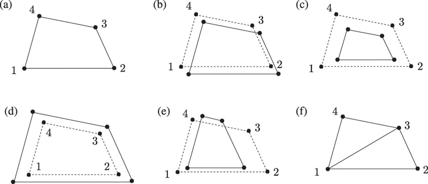
For example, Figure 1(b) shows a translation of the formation in Figure 1(a); and Figure 1(c) and (d) are uniform scaling of the formation in Figure 1(a). In particular, Figure 1(c) is a uniform contraction and Figure 1(d) is an uniform expansion. Figure 1(e) shows a non-trivial parallel formation of Figure 1(a), because the formation in Figure 1(e) cannot be obtained from the formation in Figure 1(a) by translation or uniform scaling although all the corresponding links in these two formations are parallel to each other.

Definition: parallel rigid motion

A parallel rigid motion is a trajectory along which point formations contained in this trajectory are translations or dilations of each other.

Two point formations ${\mathcal{F}}_{\mathit{p}}$, and ${\mathcal{F}}_{\mathit{q}}$, are parallel if they have the same graph and their corresponding maintenance links are parallel to each other.

Definition: parallel rigid

A formation $F(\mathit{p})$ with direction constraints is called parallel rigid if all parallel point formations of $F(\mathit{p})$ are trivially parallel to $F(\mathit{p})$. Otherwise it is called flexible.

If parallel rigid motions are the only possible trajectories then the formation is called parallel rigid, otherwise parallel flexible.

For example, the formation in Figure 1(a) is flexible. On the other hand, the formation in Figure 1(f), which is obtained from the formation in Figure 1(a) by inserting an extra link $(1,3)$, is a parallel rigid formation.

Taking the derivative of $(1)$ (recall that $\mathit{p}$ is a fixed point set and $s(t)$ is time varying in $(1)$), we obtain

$$(p_i-p_j{)}^{\perp }\cdot ({\dot{s}}_i(t)-{\dot{s}}_j(t))=0,(i,j)\in \mathcal{E},t⩾0.$$

These equations can be rewritten in matrix form as

$$R_{\mathcal{B}}(\mathit{p})\dot{s}=0$$

where $\dot{\mathit{q}}=[{\dot{q}}_1,{\dot{q}}_2,\cdots ,{\dot{q}}_n{]}^{\mathrm{\top }}$ and $R_{\mathcal{B}}(\mathit{p})$ is the rigidity matrix for formations with bearing information.

It is shown that any statement for a point formation of distances can be given for the same point formation of directions where distances are switched with directions. The isomorphism goes down the pairs of columns for each vertex, turning all the vectors by ${90}^{\circ }$ (in a direction of choice). This process preserves the solution space (just turning the solutions by ${90}^{\circ }$ as well), and turns each row for a distance into a row for a direction. Because of this geometric switching, there is a generic switching theorem that converts results in a direct fashion, so the generic type of rigidity is defined in the same manner as in the case of distances. Thus the graph theoretic test is given with the following theorem:

Theorem 1

A graph $\mathcal{G}=(\mathcal{V},\mathcal{E})$, where $\mathcal{E}$ denotes the set of links with bearing measurements, is generically parallel rigid in $2$-space if and only if there is a subset ${\mathcal{E}}^{\prime }\subseteq \mathcal{E}$ satisfying the following two conditions:

1. $|{\mathcal{E}}^{\prime }|=2|\mathcal{V}|-3$;
2. For all ${\mathcal{E}}^{″}\subseteq {\mathcal{E}}^{\prime },{\mathcal{E}}^{″}\ne \varphi ,|{\mathcal{E}}^{″}|⩽2|\mathcal{V}({\mathcal{E}}^{″})|-3$, where $\mathcal{V}({\mathcal{E}}^{″})$ is the number of vertices that are end-vertices of the edges in ${\mathcal{E}}^{″}$;

For frameworks using pure distance information, the conditions for global rigidity are stronger than those for rigidity of formation with distance constraints.

For frameworks in $2$-space with bearing information between nodes, the situation is strikingly different. Because the key constraints are linear equations, if there are two non-similar parallel formations with points $p$ and $q$, then both formations are not rigid. Therefore, for these formations, parallel rigidity implies global rigidity up to similarity. In $2$-space, if we have the $2n-3$ bearings of a parallel rigid formation, and add one length, we will have a globally rigid formation. We do have a simple combinatorial characterization (counting) and fast algorithms for global rigidity.

Theorem 2

If ${\mathcal{F}}_{\mathit{p}}$ is a formation in $2$-space, then ${\mathcal{F}}_{\mathit{p}}$ is parallel rigid if and only if ${\mathcal{F}}_{\mathit{p}}$ is globally rigid under translation and dilation maps.

Details of Proof

Suppose that ${\mathcal{F}}_{\mathit{p}}$ is not globally rigid. Therefore, there is a parallel drawing ${\mathcal{F}}_{\mathit{q}}$ which is not similar to ${\mathcal{F}}_{\mathit{p}}$ as a configuration. We will show that ${\mathcal{F}}_{\mathit{p}}$ is flexible with ${\mathcal{F}}_{\mathit{q}}$ as a non-trivial parallel drawing. For all edges $(i,j)\in \mathcal{E},(p_i-p_j)$ is parallel to $(q_i-q_j)$. Therefore, $(p_i-p_j{)}^{\perp }\cdot (q_i-q_j)=0$ as required. Since ${\mathcal{F}}_{\mathit{p}}$ is not similar to ${\mathcal{F}}_{\mathit{q}}$, there is some pair $(h,k)\notin \mathcal{E}$ such that $p_h-p_k$ is not parallel to $q_h-q_k$ . Therefore, $(p_h-p_k{)}^{\perp }\cdot (q_h-q_k)\ne 0$ . This confirms that ${\mathcal{F}}_{\mathit{q}}$ is a non-trivial parallel drawing of ${\mathcal{F}}_{\mathit{p}}$.

Conversely, suppose that ${\mathcal{F}}_{\mathit{p}}$ is flexible with a non-trivial parallel drawing ${\mathcal{F}}_{\mathit{q}}$. Then ${\mathcal{F}}_{\mathit{q}}$ itself is the non-similar parallel drawing of ${\mathcal{F}}_{\mathit{p}}$ which shows it is not globally rigid.

$◻$

More generally, nodes are not confined to use their sensing and communication links for measuring distances only. We can exploit such a possibility to generate point formation that is not only locally unique but also globally unique with as few links as a minimally rigid formation.

For formations with combined distance-bearing constraints, there is the following combinatorial characterization of parallel rigidity.

Theorem 3: generically parallel rigid

With $\mathcal{L}$ for distances and $\mathcal{B}$ for bearings, a graph $\mathcal{G}=(\mathcal{V},\mathcal{L},\mathcal{B})$ is generically parallel rigid in $2$-space if and only if the following conditions hold:

1. $|\mathcal{L}|+|\mathcal{B}|=2|\mathcal{V}|-2$ ;
2. For all subsets ${\mathcal{V}}^{\prime }$ of vertices: $|{\mathcal{L}}^{\prime }|+|{\mathcal{B}}^{\prime }|⩽2|{\mathcal{V}}^{\prime }|-2$ ;
3. For all subsets ${\mathcal{V}}^{\prime }$ of at least $2$ vertices: $|{\mathcal{B}}^{\prime }|⩽2|{\mathcal{V}}^{\prime }|-3$;
4. For all subsets ${\mathcal{V}}^{\prime }$ of at least $2$ vertices: $|{\mathcal{L}}^{\prime }|⩽2|{\mathcal{V}}^{\prime }|-3$ .

TODO Proof

B. Servatius, W. Whiteley, “Constraining plane configurations in Computer Aided Design: Combinatorics of directions and lengths,” 1995, preprint, York University, North York, Ontario.

The conditions for distance-direction constraints are closely related to the conditions for parallel rigidity for distance-bearing constraints since bearing constraints can be written as direction constraints as stated in Proposition 1.

A point formation using direction-distance constraints can be unique up to translation. This will require $2|\mathcal{V}|-2$ independent constraints. For example, it is easy to see that:

1. An independent set of $2|\mathcal{V}|-3$ distances plus any single direction is an appropriate set of $2|\mathcal{V}|-2$ constraints;
2. An independent set of $2|\mathcal{V}|-3$ directions plus any single distance is an appropriate set of $2|\mathcal{V}|-2$ constraints;
3. A spanning tree, used once for distances and a second time for directions, is an appropriate set of $2(|\mathcal{V}|-1)=2|\mathcal{V}|-2$ constraints.

A tree is a graph in which any two vertices are connected by exactly one path. Given a connected, undirected graph, a spanning tree of that graph is a subgraph which is a tree and connects all the vertices together.

Are these sufficient? Even for distances, we know that these conditions are not sufficient for special positions of the points. However, by Laman’s Theorem, they are sufficient for distances on ‘generic configurations’. The most we can expect is that these expanded conditions are also sufficient for ‘generic configurations’. We replace the entries for the points $p$, in the matrix by algebraically independent values, and look at the solution space for these values. If all solutions are translations, then almost all configurations (an open dense subset of configurations) $p\in {\mathbb{R}}^{2|\mathcal{V}|}$ have only translations. Specifically, if we use variables for the coordinates, the rank of this matrix is determined by maximal non-zero minors a finite set of polynomials in these variables. Such a polynomial is either always zero or is non-zero for an open dense subset. The intersection of this finite collection of subsets for all maximal non-zero minors forms the set of generic plane configurations for formations with distance-direction constraints.

This characterization also covers the distance-bearing combinations that permit more than one distance. Note that this is the criterion for rigidity up to translation, not for global rigidity, if there are multiple distance constraints. It is rigidity up to translation since rotations are not allowed because of bearing constraints. We suspect that it is probably the criterion for global rigidity, up to translation, if there are enough bearing constraints. Under this assumption, and assuming that angle of arrival is measured in trigonometric direction, we have a conjecture for global rigidity.

Conjecture 1 (in 2007)

Provided that the underlying graph constructed with the links representing bearing constraints form at least a spanning tree, then for generic formations, rigidity up to translation is equivalent to global rigidity of the formation.

Bearing Rigidity

Bearing constraints in mobile formations have $2$ major differences compared to directions used in parallel drawings.

Figure 2: Bearing Constaints v.s. Direction Constraints

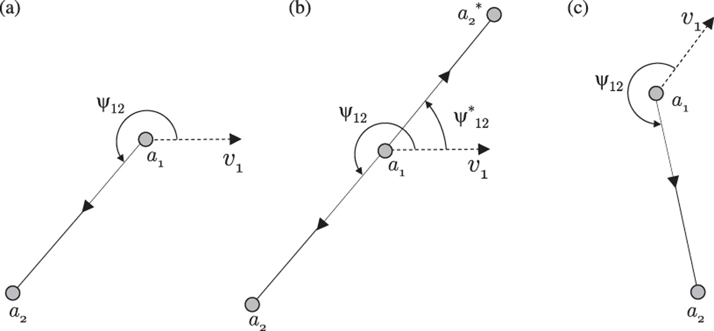
1. Bearing constraint is more stringent than direction constraint. For example, assume that $a_1$ is fixed in $2$-space as shown in Figure 2(a) and $a_2$ has a bearing constraint ${\psi }_{12}$ with $a_1$. Note that, direction constraint is satisfied by both ${\psi }_{12}$ and ${\psi }_{12}^{\ast }={\psi }_{12}-\pi$ as shown in Figure 2(b), where one is obtained by a flip of the other w.r.t. $a_1$. Thus, a direction constraint can be thought as a necessary condition of a bearing constraint. For maintaining the shape of a mobile formation, where only continuous motions of agents are feasible, flip ambiguity is avoided, and thus, we can make use of parallel drawings for the analysis and design of rigid formations that make use of bearing measurements.
2. Direction constraints, in the context of parallel drawings studied in computer-aided design, are measured w.r.t. a fixed global reference frame, whereas bearing constraints in mobile formations are measured w.r.t. the heading of leader agents. This selection of reference frame renders bearing constraints convenient for mobile formations, because follower agents act to satisfy bearing constraints as their leaders move (and possibly change their headings), hence preserving the shape of the overall formation. For example, if a1 changes its heading direction as shown in Figure 2(c), then $a_2$ has to change its position to satisfy the bearing constraint, which results in shape maintenance. This aspect makes the application of bearing rigidity in formation navigation different than the application of bearing rigidity in framework localisation.

We can state the conditions for bearing rigidity for a digraph as follows:

Definition: Bearing Rigidity

Given a digraph $\mathcal{G}(\mathcal{V},\mathcal{E})$ of a formation framework, $\mathcal{G}$ is bearing rigid if and only if there is a subset ${\mathcal{E}}^{\prime }\subseteq \mathcal{E}$ satisfying the following conditions:

1. $|{\mathcal{E}}^{\prime }|=2|\mathcal{V}|-3$;
2. For all ${\mathcal{E}}^{″}\subseteq {\mathcal{E}}^{\prime },{\mathcal{E}}^{″}\ne \varphi ,|{\mathcal{E}}^{″}|⩽2|\mathcal{V}({\mathcal{E}}^{″})|-3$, where $\mathcal{V}({\mathcal{E}}^{″})$ is the number of vertices that are end-vertices of the edges in ${\mathcal{E}}^{″}$;
3. ${\mathcal{G}}^{\prime }(\mathcal{V},{\mathcal{E}}^{\prime })$ is constraint consistent.

This test provides a combinatorial formation analysis method to test rigidity for a given formation. In the context of navigating formations of mobile agents, we will call the formations satisfying the $1^{\text{st}}$ two conditions listed above as bearing rigid formations. We will call the formations satisfying the three conditions listed above as directed bearing rigid formations. If a bearing rigid formation loses rigidity property in the loss of any edge in $\mathcal{G}$, then such a formation is called minimally (directed) bearing rigid formation.

From a formation synthesis (design) point-of-view, there is a Henneberg type method to construct bearing rigid formations.

Bearing-based Henneberg construction

A Henneberg-type construction is a technique for growing rigid digraphs starting from a single edge in 2-space. One of the following operations is applied (when applicable) at each step in the procedure. The resulting graphs are provably rigid.

• Directed $2$-valent vertex addition: Given a digraph $\mathcal{G}(\mathcal{V},\mathcal{E})$ where $(a,b)\in \mathcal{E}$, a vertex $q$ of in-degree $2$ is inserted into $\mathcal{G}$ by adding the edges $(a,q)$ and $(b,q)$.
• Directed $2$-valent vertex deletion: Given a digraph $\mathcal{G}(\mathcal{V},\mathcal{E})$ where $(a,q),(b,q)\in \mathcal{E}$, a vertex $q\in \mathcal{V}$ of in-degree $2$ with the edges $(a,q)$ and $(b,q)$ is deleted from $\mathcal{G}$.
• Directed $3$-valent vertex addition: Given a digraph $\mathcal{G}(\mathcal{V},\mathcal{E})$ where $(a,b)\in \mathcal{E}$, a vertex $q$ of in-degree $2$ and out-degree $1$ is inserted into $\mathcal{G}$ by deleting the edge $(a,b)$ and adding the edges $(a,q),(c,q)$ and $(q,b)$. This operation is also known as edge splitting operation.
• Directed $3$-valent vertex deletion: Given a digraph $\mathcal{G}(\mathcal{V},\mathcal{E})$ where $(a,q),(c,q),(q,b)\in \mathcal{E}$, the vertex $q$ of in-degree $2$ and out-degree $1$ is removed from $\mathcal{G}$ by deleting the edges $(a,q),(c,q)$ and $(q,b)$ and inserting one of the pairs in $\{(a,b),(c,b)\}$.
• Edge reversal: Given a digraph $\mathcal{G}(\mathcal{V},\mathcal{E})$ where $(a,b)\in \mathcal{E}$, an edge $(a,b)$ in $\mathcal{G}$ is replaced by $(b,a)$.

A minimally bearing rigid formation in 2-space has $2n-3$ links. Subtracted three in this formula comes from the three DoF distributed to some agents in a rigid formation: $2$ for translation and $1$ for scaling. As in the case of distance-based persistent formations, this freedom can be distributed in a number of ways.

• two-leader formation structure, in which there is an agent ( $1^{\text{st}}$ leader) that has $2$ DoF, and another agent ($2^{\text{nd}}$ leader) with $1$ DoF such that these $2$ agents are neighbours. For bearing rigid formations, we prefer the term $2$-leader formation because the agent that has $1$ DoF in a bearing rigid formation has the control of scaling on the entire formation, which makes it act like a leader rather than a follower. Moreover, by changing its bearing to the $1^{\text{st}}$ leader, the $2^{\text{nd}}$ leader can change the orientation of the entire formation.
• leader-remote follower structure, in which the agent with $1$ DoF is not a neighbour of the agent with $2$ DoF.
• three-coleaders structure. This is a formation structure in which there are three agents $a_1,a_2,a_3$ (called the coleaders) with $1$ DoF each. Three-coleader structure can further be classified within itself depending on the neighbourhood relations of coleaders.

In this article, the formations we study are of a two-leader variety.

Scalable bearing rigid formations

We need to address one more issue on bearing rigidity before we proceed any further. Bearing rigidity, as it is defined above, is based on $2n-3$ links, all of which are used for bearing constraints. An advantage of bearing rigid formations used in shape control is its uniform scalability (homothety) property, since every constraint is essentially based on an angle measurement.

However, unless there is a proper action, note that all bearing constraints will still be satisfied if a formation expands or contracts. In other words, we have no control over the scale of a formation in a bearing rigid formation. We need at least one distance measurement to be able to fix the scale of a formation, which results in ‘scalable bearing rigid formations’.

A scalable bearing rigid formation is obtained from a bearing rigid formation of $2n-3$ bearing constraints by inserting one additional distance constraint, i.e. $2n-2$ links in total. This additional distance constraint is imposed on the $2^{\text{nd}}$ leader with a new incoming link from the $1^{\text{st}}$ leader as a distance constraint. Therefore, in a scalable bearing rigid formation, the $2^{\text{nd}}$ leader has $2$ incoming links, and therefore, zero DoF when we fix the distance and bearing constraints imposed upon it. This is in contrast with a bearing rigid formation, where the $2^{\text{nd}}$ leader has only one incoming link. When we use such a single distance constraint between the $1^{\text{st}}$ leader and the $2^{\text{nd}}$ leader for shape control, all we need to do for scaling shape is to adjust this distance constraint.

In summary, the $1^{\text{st}}$ leader determines the translational motion of a formation. It has $2$ DoF. Scaling of the entire formation is managed by the $2^{\text{nd}}$ leader by adjusting its distance constraint. The rotation of the formation is achieved either by changing the heading of the $1^{\text{st}}$ leader or by changing the bearing of the $2^{\text{nd}}$ leader.

Directed Rigidity

Acyclic formations

First, we give some terminology.

• A directed edge is written with an ordered pair of end-vertices $(i,j)$ representing an edge directed from $j$ to $i$ and drawn with an arrow from $j$ to $i$, that is from the source to the sink.
• The number of edges directed into a given vertex i in a digraph $\mathcal{G}$ is called the in-degree of the vertex and is denoted by $d_{\mathcal{G}}^{-}(i)$. The number of edges directed out from a given vertex $i$ in a digraph $\mathcal{G}$ is called the out-degree of the vertex and is denoted by $d_{\mathcal{G}}^{+}(i)$.
• The out-neighborhood ${\mathcal{N}}_{\mathcal{G}}^{+}(i)$ of a vertex $i$ is $\{j\in \mathcal{V}:(j,i)\in \mathcal{E}\}$ , and the in-neighborhood ${\mathcal{N}}_{\mathcal{G}}^{-}(i)$ of a vertex $i$ is $\{j\in \mathcal{V}:(i,j)\in \mathcal{E}\}$. The union of out-neighborhood and in-neighborhood is the set of neighbors of $i$, i.e., the (open) neighborhood of $i$, ${\mathcal{N}}_{\mathcal{G}}(i)$. When $i$ is also included, it is the closed neighborhood of $i,{\mathcal{N}}_{\mathcal{G}}[i]$.

Definition: directed path

A directed path is a non-empty digraph $\mathcal{G}=(\mathcal{V},\mathcal{E})$ of the form $\mathcal{V}=\{x_0,x_1,\cdots ,x_k\},\mathcal{E}=\{(x_0,x_1),(x_1,x_2),\cdots ,(x_{k-1},x_k)\}$. We refer to a path by the sequence of its vertices as $P=x_0{x}_1\cdots x_k$ and calling $P$ a path from $x_0$ to $x_k$. In a simple path, all the $x_i$ are distinct. In a closed path, $x_0=x_k$.

Definition: cycle

A closed directed path, with no repeated vertices other than the starting and ending vertices is called a (directed) cycle and is denoted by $C$.

Definition: cycle graph & cyclic graph & acyclic graph

• A cycle graph is a graph on $n$ vertices containing a single cycle through all vertices.
• A cyclic graph is a graph containing at least one cycle.
• A graph that is not cyclic is said to be acyclic.

Care should be taken with cyclic formations, which can lead to unstable behaviours in the presence of measurement errors if the agents are not allowed to communicate. Further, we show that bearing rigid formations with coleader structure and leader-remote follower structure occur only in cyclic formations. Therefore, we avoid such structures in shape control.

Another disadvantage of coleader formations in bearing rigid formations is that they not only require a coordinated motion of three coleaders, but also require a consensus on the heading of all three coleaders. We have the following two theorems.

Theorem 0.1

For a digraph $\mathcal{G}=(\mathcal{V},\mathcal{E})$, with at least $2$ vertices, the following are equivalent:

1. $\mathcal{G}=(\mathcal{V},\mathcal{E})$ is minimally bearing rigid and acyclic;
2. $\mathcal{G}=(\mathcal{V},\mathcal{E})$ is constructed from a single edge by a sequence of directed vertex additions
3. $\mathcal{G}=(\mathcal{V},\mathcal{E})$ has two-leader architecture, and is acyclic with all other vertices having in-degree exactly $2$.

Details of Proof

1. $1\to 2$: Minimally directed bearing rigid digraphs are constraint consistent and they have $|\mathcal{E}|=2|\mathcal{V}|-3$. We are given that there are no cycles in the digraph. Therefore, the digraph represents a partial order between vertices. The partial order can be made into a complete order. The smallest element in the order is the $1^{\text{st}}$ leader, and the next smallest is the $2^{\text{nd}}$ leader, and this will be our target edge for the directed Henneberg sequence. Assume that there are more than $3$ vertices. The maximal element has all edges in so it has in-degree $d_{\mathcal{G}}^{-}(i)⩽2$. Overall, since each edge is directed: $\sum _{i\in \mathcal{V}}{d}_{\mathcal{G}}^{-}(i)=|\mathcal{E}|=2|\mathcal{V}|-3$. However, the two initial vertices have a total in-degree of $1$, so on all other vertices ${\mathcal{V}}^{\prime }:\sum _{i\in {\mathcal{V}}^{\prime }}{d}_{\mathcal{G}}^{-}(i)=|\mathcal{E}|=2|{\mathcal{V}}^{\prime }|=2(|\mathcal{V}|-2)$. We also know that all vertices have $d_{\mathcal{G}}^{-}(i)⩽2$, so we conclude that all other vertices have $d_{\mathcal{G}}^{-}(i)=2$. Take the maximal vertex in the linear order. All edges are in-directed, so the overall valence is $2$. We can apply $2$-valent vertex deletion to get a smaller directed bearing rigid acyclic graph, with the induced linear order. We continue with this until there are only the $1^{\text{st}}$ leader and the $2^{\text{nd}}$ leader. Reversing this sequence gives the desired construction.
2. $2$ is equivalent to $3$: This is immediate, as the initial edge is the first leader-second leader edge, and the valence assumption is equivalent to the count of $2$.
   $◻$

Theorem 0.2

Minimal bearing rigid formations with coleader structure or leader-remote follower structure occur only in cyclic formations.

Proof: Suppose that coleader structures and leader-remote follower structures occur in acyclic formations too. Acyclic formations can be built by using only $2$-valent vertex addition and creates topological order of vertices from Theorem 0.1. Apply $2$-valent vertex deletion to the formation in reverse order until we are left with a single edge. There is $1$ vertex of in-degree $0$ (having $2$ DoF left) and $1$ vertex of in-degree $1$ (having 1 DoF left). Thus, these two agents manage all the DoF that the formation has, which is $3$, leaving no DoF to the rest of the agents. Thus, all the remaining vertices have an in-degree $2$, which means that the acyclic formation has two-leader architecture. This contradicts with our initial assumption. Thus, coleader structures or leader-remote follower structures occur only in cyclic formations.

$◻$

In short, formation control using bearing measurements is straightforward if the underlying directed graph is acyclic, since it is based on a partial ordering of agents due to an absence of cycles. Acyclic bearing rigid formations can be constructed using a sequence of directed vertex additions, and they have two-leader architecture. Therefore, we will base the rest of this article on acyclic bearing rigid formations. In particular, we will make use of scalable bearing rigid formations. Construction of such formations starts with a double edge between the $1^{\text{st}}$ leader and the $2^{\text{nd}}$ leader (one distance constraint-one bearing constraint), then continues with directed $2$-valent vertex additions with bearing constraints.

$2$-directed digraphs

Any ordinary node in a framework with directed bearing links needs to have at least $2$ in-coming links to localize itself, that is, $d_{\mathcal{G}}^{-}(i)⩾2$. Of course, anchor nodes do not need any in-coming links to localize themselves.

However, we insert the implicit links among anchor nodes to obtain the grounded graph. Furthermore, the existence of one anchor node rules out translation. If there is only one anchor node, then scaling is still allowed. This means that $1$ ordinary node can have $1$ DoF. We call such a node a free node. Anchor node and free node together make up the set of guide nodes. The digraph $\mathcal{G}=(\mathcal{V},\mathcal{E})$ is $2$-directed if for all $i\in \mathcal{V},d_{\mathcal{G}}^{-}(i)⩽2$.

A point formation with directed bearing constraints is called directed parallel rigid if all directed parallel point formations are trivially parallel. There are a number of issues that must be addressed in the localization of frameworks with directed links. We identify three key layers as follows:

1. Parallel rigidity of the underlying undirected formation;
2. Directed parallel rigidity of the formation;
3. Convergence and the quality of initial position estimates in the framework

If underlying undirected formation is non-rigid, then directed formation cannot be rigid. Thus, undirected rigidity is a necessary condition for directed rigidity. On the other hand, when we associate a direction to each link in a rigid undirected formation, directed parallel rigidity is not necessarily guaranteed, because an in-degree of a node may be set to $1$ while another node has an in-degree of $3$ resulting from a poor selection of directions. Consequently, undirected parallel rigidity is not a sufficient condition for directed parallel rigidity. Even if there is subset of the grounded graph that is $2$-directed, the undirected graph may still be flexible. Thus, we can state the conditions for global rigidity for a directed graph as follows:

Theorem 4

Given a grounded digraph $\hat{\mathcal{G}}=(\mathcal{V},\hat{\mathcal{B}})$ of the framework $N$, there is a subset ${\mathcal{B}}^{\prime }\subseteq \mathcal{B}$ satisfying the following conditions:

1. $|{\mathcal{B}}^{\prime }|=2|\mathcal{V}|-3$;
2. For all ${\mathcal{B}}^{″}\subseteq {\mathcal{B}}^{\prime },{\mathcal{B}}^{″}\ne \varphi ,|{\mathcal{B}}^{″}|⩽2|\mathcal{V}({\mathcal{B}}^{″})|-3$, where $\mathcal{V}({\mathcal{B}}^{″})$ is the number of vertices that are end-vertices of the edges in ${\mathcal{B}}^{″}$;
3. ${\mathcal{G}}^{\prime }(\mathcal{V},{\mathcal{B}}^{\prime })$ is $2$-directed.

Bearing Rigidity in Arbitary Dimensions [4]

Basic Conceptions

Define:

$$e_{ij}\triangleq p_j-p_i,g_{ij}\triangleq \frac{e_{ij}}{\parallel e_{ij}\parallel }=\frac{p_j-p_i}{\parallel p_j-p_i\parallel },\mathrm{\forall }(i,j)\in \mathcal{E}.$$

Note the unit vector $g_{ij}$ represents the relative bearing of $p_j$ to $p_i$. This unit-vector representation is different from the conventional ways where a bearing is described as one angle (azimuth) in ${\mathbb{R}}^2$, or two angles (azimuth and altitude) in ${\mathbb{R}}^3$. Note also that $e_{ij}=-e_{ji}$ and $g_{ij}=-g_{ji}$.

We now introduce an important orthogonal projection operator that will be widely used in this paper. For any nonzero vector $\mathit{x}\in {\mathbb{R}}^d(d⩾2)$, define the operator $P:{\mathbb{R}}^d⟼{\mathbb{R}}^{d\times d}$ as

$$P(\mathit{x})\triangleq I_d-\frac{\mathit{x}}{\parallel \mathit{x}\parallel }\frac{{\mathit{x}}^{\mathrm{\top }}}{\parallel \mathit{x}\parallel }$$

For notational simplicity, denote $P_x=P(\mathit{x})$. Note:

• $P_x$ is an orthogonal projection matrix which geometrically projects any vector onto the orthogonal compliment of $\mathit{x}$
• It can be verified that $P_x^{\mathrm{\top }}=P_x,P_x^2=P_x$, and $P_x$ is positive semi-definite.
• $\mathrm{Null}(P_x)=\mathrm{span}\{\mathit{x}\}$ and the eigenvalues of $P_x$ are $\{0,1^{(d-1)}\}$.
• Any two unit vectors $\mathit{x},\mathit{y}\in {\mathbb{R}}^d$ satisfy ${\mathit{x}}^{\mathrm{\top }}{P}_y\mathit{x}={\mathit{y}}^{\mathrm{\top }}{P}_x\mathit{y}$.
• For any nonzero vectors ${\mathit{x}}_1,\cdots ,{\mathit{x}}_n\in {\mathbb{R}}^d$ where $n⩾2,d⩾2$, the matrix $\sum _{i=1}^n{P}_{x_i}\in {\mathbb{R}}^{d\times d}$ is nonsingular if and only if at least two of ${\mathit{x}}_1,\cdots ,{\mathit{x}}_n$ are not colinear
• For any two nonzero vectors $x,y\in {\mathbb{R}}^d$, if $\theta \in [0,\pi ]$ is the angle between them so that ${\mathit{x}}^{\mathrm{\top }}\mathit{y}=\parallel \mathit{x}\parallel \parallel \mathit{y}\parallel \cos \theta$, then $\parallel P_x-P_y\parallel =\sin \theta$
• If $\mathit{x}\in {\mathbb{R}}^3$ is a unit vector, then $P_x=-[\mathit{x}{]}_{\times }^2$ where

$$[\mathit{x}{]}_{\times }=\left[\begin{array}{ccc}0& -x_3& x_2\\ x_3& 0& -x_1\\ -x_2& x_1& 0\end{array}\right]\in {\mathbb{R}}^{3\times 3}$$

is the skew-symmetric matrix associated with $\mathit{x}$

Lemma 1: parallel in $d$-dimensions

Two nonzero vectors $\mathit{x},\mathit{y}\in {\mathbb{R}}^d$ are parallel if and only if $P_x\mathit{y}=0$ (or equivalently $P_y\mathit{x}=0$).

Proof: The result follows from $\mathrm{Null}(P_x)=\mathrm{span}\{\mathit{x}\}$.

$◻$

Figure 3: An illustration of the orthogonal projection matrix.

Most existing works, like the last section, use the notion of normal vectors to describe parallel vectors in ${\mathbb{R}}^2$. Specifically, given a nonzero vector $\mathit{x}\in {\mathbb{R}}^2$, denote ${\mathit{x}}^{\perp }\in {\mathbb{R}}^2$ as a nonzero normal vector satisfying ${\mathit{x}}^{\mathrm{\top }}{\mathit{x}}^{\perp }=0$. Then any vector $\mathit{y}\in {\mathbb{R}}^2$ is parallel to $\mathit{x}$ if and only if $({\mathit{x}}^{\perp }{)}^{\mathrm{\top }}\mathit{y}=0$. This approach is applicable to 2D cases but difficult to extend to arbitrary dimensions. Moreover, it is straightforward to prove that in ${\mathbb{R}}^2$ the use of the orthogonal projection operator is equivalent to the use of normal vectors based on the fact that

$$P_x=\frac{{\mathit{x}}^{\perp }({\mathit{x}}^{\perp }{)}^{\mathrm{\top }}}{\parallel {\mathit{x}}^{\perp }{\parallel }^2},\mathrm{\forall }\mathit{x}\in {\mathbb{R}}^2.$$

Fundamental Concepts about Bearing Rigidity

Now ready to define the fundamental concepts in bearing rigidity. These concepts are defined analogously to those in the distance rigidity theory.

Definition: Bearing Equivalency

Frameworks $\mathcal{G}(\mathit{p})$ and $\mathcal{G}({\mathit{p}}^{\prime })$ are bearing equivalent if $P_{(p_i-p_j)}(p_i^{\prime }-p_j^{\prime })=0$ for all $(i,j)\in \mathcal{E}$.

Definition: Bearing Congruency

Frameworks $\mathcal{G}(\mathit{p})$ and $\mathcal{G}({\mathit{p}}^{\prime })$ are bearing congruency if $P_{(p_i-p_j)}(p_i^{\prime }-p_j^{\prime })=0$ for all $i,j\in \mathcal{V}$.

By definition, bearing congruency implies bearing equivalency. The converse, however, is not true, as illustrated in Figure 4.

Figure 4: Bearing equivalent but not bearing congruent

Definition: Global Bearing Rigidity

A framework $\mathcal{G}(\mathit{p})$ is globally bearing rigid if an arbitrary framework that is bearing equivalent to $\mathcal{G}(\mathit{p})$ is also bearing congruent to $\mathcal{G}(\mathit{p})$.

By definition, global bearing rigidity implies bearing rigidity. As will be shown later, the converse is also true.

We next define infinitesimal bearing rigidity, which is one of the most important concepts in the bearing rigidity theory. Consider an arbitrary orientation of the graph $\mathcal{G}$ and denote

$$e_k\triangleq p_j-p_i,g_k\triangleq \frac{e_k}{\parallel e_k\parallel }=\frac{p_j-p_i}{\parallel p_j-p_i\parallel },\mathrm{\forall }k\in \{1,2,\cdots ,m\}.$$

as the edge vector and the bearing for the $k$-th directed edge. Note that $g_k$ is the unit vector so that $P(g_{ij})=I_d-g_{ij}{g}_{ij}^{\mathrm{\top }}$. Denote $\mathit{z}=[e_1^{\mathrm{\top }},\cdots ,e_m^{\mathrm{\top }}{]}^{\mathrm{\top }}$ and $\mathit{g}=[g_1^{\mathrm{\top }},\cdots ,g_m^{\mathrm{\top }}{]}^{\mathrm{\top }}$. Note $\mathit{z}$ satisfies $\mathit{z}=\overline{H}\mathit{p}$ where $\overline{H}=H\otimes I_d$ and $H$ is the incidence matrix of the graph.. Define the bearing rigidity function $B_{\mathcal{G}}(\mathit{p}):{\mathbb{R}}^{dn}⟼{\mathbb{R}}^{dm}$ as

$$B_{\mathcal{G}}(\mathit{p})\triangleq [g_1^{\mathrm{\top }},\cdots ,g_m^{\mathrm{\top }}{]}^{\mathrm{\top }}\in {\mathbb{R}}^{dm}.$$

The bearing function describes all the bearings in the framework. The bearing rigidity matrix is defined as the Jacobian of the bearing rigidity function

$$\begin{array}{}\text{(2)}& R_{\mathcal{B}}(\mathit{p})\triangleq \frac{\partial B_{\mathcal{G}}(\mathit{p})}{\partial \mathit{p}}\in {\mathbb{R}}^{dm\times dn}.\end{array}$$

Let $\delta \mathit{p}$ be a variation of the configuration $\mathit{p}$. If $R(p)\delta \mathit{p}=\mathbf{0}$, then $\delta \mathit{p}$ is called an infinitesimal bearing motion of $\mathcal{G}(\mathit{p})$. This is analogous to infinitesimal motions in distance-based rigidity.

• The term infinitesimal is due to the fact that the bearing rigidity matrix is the first-order derivative (the Jacobian) of the bearing vectors w.r.t. the positions of the nodes.
• An infinitesimal bearing motion of a framework is a motion of some nodes that preserves all of the bearings. All of the infinitesimal bearing motions of a framework form the null space of the bearing rigidity matrix

Distance preserving motions of a framework include rigid-body translations and rotations, whereas bearing preserving motions of a framework include translations and scalings.

An infinitesimal bearing motion is called trivial if it corresponds to a translation and a scaling of the entire framework.

Definition: Infinitesimal Bearing Rigidity

A framework is infinitesimally bearing rigid if all the infinitesimal bearing motions are trivial.

One important property of an infinitesimally bearing rigid framework is that its shape can be uniquely determined by the inter-neighbor bearings.

An alternative necessary and sufficient condition for infinitesimal bearing rigidity is based on a special matrix termed the bearing Laplacian. [5,6]

Definition: Bearing Laplacian of Networks

Given the framework $(\mathcal{G},\mathit{p})$ with no colocated nodes, define the bearing Laplacian $L_{\mathcal{B}}\in {\mathbb{R}}^{dn\times dn}$ as

$$[L_{\mathcal{B}}{]}_{ij}=\{\begin{array}{ll}{\mathbf{0}}_{d\times d},& i\ne j,(i,j)\notin \mathcal{E}\\ -P_{g_{ij}},& i\ne j,(i,j)\in \mathcal{E}\\ \sum _{k\in {\mathcal{N}}_i}{P}_{g_{ik}},& i=j,(i,j)\in \mathcal{V}\end{array}$$

where $[L_{\mathcal{B}}{]}_{ij}$ is the $ij$-th block of submatrix of $L_{\mathcal{B}}$.

The bearing Laplacian of a framework can be viewed as a weighted graph Laplacian matrix with weights that are matrices, which describes both the underlying graph and the interneighbor bearings of the framework. Thus, the bearing Laplacian describes not only the topological structure of the framework but the values of the edge bearings.

For a framework with an undirected graph, the bearing Laplacian has the same rank and null space as the bearing rigidity matrix. When the underlying graph is directed, the bearing Laplacian and the bearing rigidity matrix may have different ranks and null spaces (See Bearing Persistence part for details). Compared to the bearing rigidity matrix, the bearing Laplacian is more convenient to use because it is symmetric and positive semidefinite for undirected graphs. Here is more specific:

Lemma 2

For a framework $\mathcal{G}(\mathit{p})$ with undirected graph $\mathcal{G}$, the bearing Laplacian $L_{\mathcal{B}}$ satisfies the following:

1. $L_{\mathcal{B}}$ is symmetric positive semi-definite;
2. $\mathrm{rank}(L_{\mathcal{B}})⩽dn-d-1$ and $\mathrm{span}\{\mathbf{1}\otimes I_d,\mathit{p}\}\subseteq Null(L_{\mathcal{B}})$;
3. $\mathrm{rank}(L_{\mathcal{B}})=dn-d-1$ and $\mathrm{Null}(L_{\mathcal{B}})=\mathrm{span}\{\mathbf{1}\otimes I_d,\mathit{p}\}$ if and only if $\mathcal{G}(\mathit{p})$ is infinitesimally bearing rigid.

Details of Proof

Assign an arbitrary orientation to each undirected edge and label the edge vectors and bearings for the directed edges as $\{e_k{\}}_{k=1}^m$ and $\{g_k{\}}_{k=1}^m$, respectively. Then the bearing Laplacian $L_{\mathcal{B}}$ can be expressed as $L_{\mathcal{B}}={\overline{H}}^{\mathrm{\top }}\mathrm{diag}(P_{g_k})\overline{H}$. It further follows from $P_{g_k}=P_{g_k}^{\mathrm{\top }}{P}_{g_k}$ that

$$L_{\mathcal{B}}={\overline{H}}^{\mathrm{\top }}\mathrm{diag}(P_{g_k})\overline{H}\triangleq R^{\mathrm{\top }}R$$

Note $R=\mathrm{diag}(\parallel e_k\parallel I_d)R_{\mathcal{B}}$ where $R_{\mathcal{B}}$ is the bearing rigidity matrix. As a result, the matrix $R$ and hence $L_{\mathcal{B}}$, have exactly the same rank and null space as $R_{\mathcal{B}}$. Then the results in $2^{\text{nd}}$ and $3^{\text{rd}}$ follow immediately from Lemma 5 and Theorem 8.

$◻$

Since the nodes in the framework are partitioned into anchors and followers, it will be useful to partition the corresponding bearing Laplacian as

$$L_{\mathcal{B}}=\left[\begin{array}{cc}{L}_{{\mathcal{B}}_{aa}}& L_{{\mathcal{B}}_{af}}\\ L_{{\mathcal{B}}_{fa}}& L_{{\mathcal{B}}_{ff}}\end{array}\right]$$

where $L_{{\mathcal{B}}_{aa}}\in {\mathbb{R}}^{d{n}_a\times d{n}_a},L_{{\mathcal{B}}_{af}}=L_{{\mathcal{B}}_{fa}}^{\mathrm{\top }}\in {\mathbb{R}}^{d{n}_a\times d{n}_f},L_{{\mathcal{B}}_{ff}}\in {\mathbb{R}}^{d{n}_f\times d{n}_f}$

Lemma 3

For any framework $\mathcal{G}(p)$ with undirected graph $\mathcal{G}$, the subblock matrix $L_{{\mathcal{B}}_{ff}}$ is symmetric positive semi-definite and satisfies $L_{{\mathcal{B}}_{ff}}{p}_f+L_{{\mathcal{B}}_{fa}}{p}_a=\mathbf{0}$.

Details of Proof

For any nonzero $\mathit{x}\in {\mathbb{R}}^{d{n}_f}$, denote $\overline{\mathit{x}}=[0,{\mathit{x}}^{\mathrm{\top }}{]}^{\mathrm{\top }}\in {\mathbb{R}}^{dn}$. Since $L_{\mathcal{B}}⪰0$, we have ${\mathit{x}}^{\mathrm{\top }}{L}_{{\mathcal{B}}_{ff}}\mathit{x}={\overline{\mathit{x}}}^{\mathrm{\top }}{L}_{\mathcal{B}}\overline{\mathit{x}}⩾0$. As a result, $L_{{\mathcal{B}}_{ff}}$ is positive semi-definite. Since $\mathit{p}\in \mathrm{Null}(L_{\mathcal{B}})$ as suggested by Lemma 2, we have $L_{\mathcal{B}}\mathit{p}=\mathbf{0}$ which further implies $L_{{\mathcal{B}}_{ff}}{p}_f+L_{{\mathcal{B}}_{fa}}{p}_a=\mathbf{0}$.

$◻$

Up to this point, we have introduced all the fundamental concepts in the bearing rigidity theory. We next explore the properties of these concepts. We first derive a useful expression for the bearing rigidity matrix.

Relationship among types of bearing rigidity

Lemma 4

The bearing rigidity matrix $R_{\mathcal{B}}(\mathit{p})$ in $(2)$ can be expressed as

$$\begin{array}{}\text{(3)}& R_{\mathcal{B}}(\mathit{p})=\mathrm{diag}\left(\frac{P_{g_k}}{\parallel e_k\parallel }\right)\overline{H}.\end{array}$$

Details of Proof

It follows from $g_k=e_k/\parallel e_k\parallel \mathrm{\forall }k\in \{1,2,\cdots ,m\}$ that:

$$\frac{\partial g_k}{\partial e_k}=\frac{1}{\parallel e_k\parallel }(I_d-\frac{e_k}{\parallel e_k\parallel }\frac{e_k^{\mathrm{\top }}}{\parallel e_k\parallel })=\frac{1}{\parallel e_k\parallel }{P}_{g_k}.$$

As a result, $\partial B_{\mathcal{G}}(\mathit{p})/\partial \mathit{z}=\mathrm{diag}(P_{g_k}/\parallel e_k\parallel )$ and consequently

$$R_{\mathcal{B}}(\mathit{p})=\frac{\partial B_{\mathcal{G}}(\mathit{p})}{\partial \mathit{z}}\frac{\partial \mathit{z}}{\partial \mathit{p}}=\mathrm{diag}\left(\frac{P_{g_k}}{\parallel e_k\parallel }\right)\overline{H}.$$

Q.E.D.

$◻$

The expression $(3)$ can be used to characterize the null space and the rank of the bearing rigidity matrix.

Lemma 5

A framework $\mathcal{G}(\mathit{p})$ in ${\mathbb{R}}^d$ always satisfies:

• $\mathrm{span}\{\mathbf{1}\otimes I_d,\mathit{p}\}\subseteq \mathrm{Null}(R_{\mathcal{B}}(\mathit{p}))$
• $\mathrm{rank}(R_{\mathcal{B}}(\mathit{p}))⩽dn-d-1$.

Details of Proof

1. It's clear that $\mathrm{span}\{\mathbf{1}\otimes I_d\}\subseteq \mathrm{Null}(\overline{H})\subseteq \mathrm{Null}(R_{\mathcal{B}}(\mathit{p}))$
2. Since $P_{e_k}{e}_k=0$, we have $R_{\mathcal{B}}(\mathit{p})\mathit{p}=\mathrm{diag}\left(\frac{P_{g_k}}{\parallel e_k\parallel }\right)\overline{H}\mathit{p}=\mathrm{diag}\left(\frac{P_{g_k}}{\parallel e_k\parallel }\right)\mathit{z}=0$ and hence $\mathit{p}\subseteq \mathrm{Null}(R_{\mathcal{B}}(\mathit{p}))$.
3. The inequality $\mathrm{rank}(R_{\mathcal{B}}(\mathit{p}))⩽dn-d-1$ follows immediately from $\mathrm{span}\{\mathbf{1}\otimes I_d,\mathit{p}\}\subseteq \mathrm{Null}(R_{\mathcal{B}}(\mathit{p}))$.
   $◻$

For any undirected graph $\mathcal{G}=(\mathcal{V},\mathcal{E})$, denote ${\mathcal{G}}^{\mathcal{K}}$ as the complete graph over the same vertex set $\mathcal{V}$, and $R_{\mathcal{B}}^{\mathcal{K}}(\mathit{p})$ as the bearing rigidity matrix of the framework ${\mathcal{G}}^{\mathcal{K}}(\mathit{p})$. The next result gives the necessary and sufficient conditions for bearing equivalency and bearing congruency.

Theorem 5: bearing equivalent & bearing congruent

Two frameworks $\mathcal{G}(\mathit{p})$ and $\mathcal{G}({\mathit{p}}^{\prime })$ are:

• bearing equivalent if and only if $R_{\mathcal{B}}(\mathit{p}){\mathit{p}}^{\prime }=\mathbf{0}$,
• bearing congruent if and only if $R_{\mathcal{B}}^{\mathcal{K}}(\mathit{p}){\mathit{p}}^{\prime }=\mathbf{0}$.

Details of Proof

Since $R_{\mathcal{B}}(\mathit{p}){\mathit{p}}^{\prime }=\mathrm{diag}\left(\frac{P_{g_k}}{\parallel e_k\parallel }\right)\overline{H}{\mathit{p}}^{\prime }=\mathrm{diag}\left(\frac{P_{g_k}}{\parallel e_k\parallel }\right)\mathrm{diag}(P_{g_k}){\mathit{z}}^{\prime }$, we have

$$R_{\mathcal{B}}(\mathit{p}){\mathit{p}}^{\prime }=\mathbf{0}\iff P_{g_k}{e}_k^{\prime }=0,\mathrm{\forall }k\in \{1,\cdots ,m\}.$$

Therefore, by Definition of bearing equivalent, the two frameworks are bearing equivalent if and only if $R_{\mathcal{B}}(\mathit{p}){\mathit{p}}^{\prime }=\mathbf{0}$. By Definition of bearing equivalent, it can be analogously shown that frameworks are bearing equivalent if and only if $R_{\mathcal{B}}^{\mathcal{K}}(\mathit{p}){\mathit{p}}^{\prime }=\mathbf{0}$.

$◻$

Since any infinitesimal motion $\delta \mathit{p}$ is in $\mathrm{Null}(R_{\mathcal{B}}(\mathit{p}))$, it is implied from Lemma 5 and Theorem 5 that $R_{\mathcal{B}}(\mathit{p})(\mathit{p}+\delta \mathit{p})=\mathbf{0}$ and hence $\mathcal{G}(\mathit{p}+\delta \mathit{p})$ is bearing equivalent to $\mathcal{G}(\mathit{p})$.

We next give a useful lemma and then prove the necessary and sufficient condition for global bearing rigidity.

Lemma 6

A framework $\mathcal{G}(\mathit{p})$ in ${\mathbb{R}}^d$ always satisfies:

• $\mathrm{span}\{\mathbf{1}\otimes I_d,\mathit{p}\}\subseteq \mathrm{Null}(R_{\mathcal{B}}^{\mathcal{K}}(\mathit{p}))\subseteq \mathrm{Null}(R_{\mathcal{B}}(\mathit{p}))$
• $\mathrm{rank}(R_{\mathcal{B}}(\mathit{p}))⩽\mathrm{rank}(R_{\mathcal{B}}^{\mathcal{K}}(\mathit{p}))⩽dn-d-1$.

Details of Proof

1. The result that $\mathrm{span}\{\mathbf{1}\otimes I_d,\mathit{p}\}\subseteq \mathrm{Null}(R_{\mathcal{B}}^{\mathcal{K}}(\mathit{p}))$ and $\mathrm{rank}(R_{\mathcal{B}}^{\mathcal{K}}(\mathit{p}))⩽dn-d-1$ can be proved similarly as Lemma 5.
2. For any $\delta \mathit{p}\in \mathrm{Null}(R_{\mathcal{B}}^{\mathcal{K}}(\mathit{p}))$, we have $R_{\mathcal{B}}^{\mathcal{K}}(\mathit{p})\delta \mathit{p}=\mathbf{0}\Rightarrow R_{\mathcal{B}}^{\mathcal{K}}(\mathit{p})(\mathit{p}+\delta \mathit{p})=\mathbf{0}$. As a result, $\mathcal{G}(\mathit{p}+\delta \mathit{p})$ is bearing congruent to $\mathcal{G}(\mathit{p})$ by Theorem 5. Since bearing congruency implies bearing equivalency, we further know $R_{\mathcal{B}}(\mathit{p})(\mathit{p}+\delta \mathit{p})=\mathbf{0}$ and hence $R_{\mathcal{B}}(\mathit{p})\delta \mathit{p}=\mathbf{0}$. Therefore, any $\delta \mathit{p}$ in $\mathrm{Null}(R_{\mathcal{B}}^{\mathcal{K}}(\mathit{p}))$ is also in $\mathrm{Null}(R_{\mathcal{B}}(\mathit{p}))$.
3. Since $R_{\mathcal{B}}(\mathit{p}),R_{\mathcal{B}}^{\mathcal{K}}(\mathit{p})$ have the same column number, it follows immediately that $\mathrm{rank}(R_{\mathcal{B}}(\mathit{p}))⩽\mathrm{rank}(R_{\mathcal{B}}^{\mathcal{K}}(\mathit{p}))$.
   $◻$

Theorem 6: Condition for Global Bearing Rigidity

A framework $\mathcal{G}(\mathit{p})$ in ${\mathbb{R}}^d$ is globally bearing rigid if and only if $\mathrm{Null}(R_{\mathcal{B}}^{\mathcal{K}}(\mathit{p}))=\mathrm{Null}(R_{\mathcal{B}}(\mathit{p}))$ or equivalently $\mathrm{rank}(R_{\mathcal{B}}^{\mathcal{K}}(\mathit{p}))=\mathrm{rank}(R_{\mathcal{B}}(\mathit{p}))$.

Details of Proof

1. (Necessity) Suppose the framework $\mathcal{G}(\mathit{p})$ is globally bearing rigid. We next show that $\mathrm{Null}(R_{\mathcal{B}}(\mathit{p}))\subseteq \mathrm{Null}(R_{\mathcal{B}}^{\mathcal{K}}(\mathit{p}))$. For any $\delta \mathit{p}\in \mathrm{Null}(R_{\mathcal{B}}(\mathit{p}))$, we have $R_{\mathcal{B}}(\mathit{p})\delta \mathit{p}=\mathbf{0}\Rightarrow R_{\mathcal{B}}(\mathit{p})(\mathit{p}+\delta \mathit{p})=\mathbf{0}$. As a result, $\mathcal{G}(\mathit{p}+\delta \mathit{p})$ is bearing equivalent to $\mathcal{G}(\mathit{p})$ according to Theorem 5. Since $\mathcal{G}(\mathit{p})$ is globally bearing rigid, it follows that $\mathcal{G}(\mathit{p}+\delta \mathit{p})$ is also bearing congruent to $\mathcal{G}(\mathit{p})$, which means $R_{\mathcal{B}}^{\mathcal{K}}(p)(p+\delta \mathit{p})=\mathbf{0}\Rightarrow R_{\mathcal{B}}^{\mathcal{K}}(p)\delta \mathit{p}=\mathbf{0}$. Therefore, any $\delta \mathit{p}$ in $\mathrm{Null}(R_{\mathcal{B}}(\mathit{p}))$ is in $\mathrm{Null}(R_{\mathcal{B}}^{\mathcal{K}}(\mathit{p}))$ and thus $\mathrm{Null}(R_{\mathcal{B}}(\mathit{p}))\subseteq \mathrm{Null}(R_{\mathcal{B}}^{\mathcal{K}}(\mathit{p}))$. Since $\mathrm{Null}(R_{\mathcal{B}}^{\mathcal{K}}(\mathit{p}))\subseteq \mathrm{Null}(R_{\mathcal{B}}(\mathit{p}))$ as shown in Lemma 6, we have $\mathrm{Null}(R_{\mathcal{B}}(\mathit{p}))=\mathrm{Null}(R_{\mathcal{B}}^{\mathcal{K}}(\mathit{p}))$.
2. (Sufficiency) Suppose $\mathrm{Null}(R_{\mathcal{B}}(\mathit{p}))=\mathrm{Null}(R_{\mathcal{B}}^{\mathcal{K}}(\mathit{p}))$. Any framework $\mathcal{G}({\mathit{p}}^{\prime })$ that is bearing equivalent to $\mathcal{G}(\mathit{p})$ satisfies $R_{\mathcal{B}}(\mathit{p}){\mathit{p}}^{\prime }=\mathbf{0}$. It then follows from $\mathrm{Null}(R_{\mathcal{B}}(\mathit{p}))=\mathrm{Null}(R_{\mathcal{B}}^{\mathcal{K}}(\mathit{p}))$ that $R_{\mathcal{B}}^{\mathcal{K}}(\mathit{p}){\mathit{p}}^{\prime }=\mathbf{0}$, which means $\mathcal{G}({\mathit{p}}^{\prime })$ is also bearing congruent to $\mathcal{G}(\mathit{p})$. As a result, $\mathcal{G}(\mathit{p})$ is globally bearing rigid.
3. Because $R_{\mathcal{B}}(\mathit{p})$ and $R_{\mathcal{B}}^{\mathcal{K}}(\mathit{p})$ have the same column number, it follows immediately that $\mathrm{Null}(R_{\mathcal{B}}^{\mathcal{K}}(\mathit{p}))=\mathrm{Null}(R_{\mathcal{B}}(\mathit{p}))$ if and only if $\mathrm{rank}(R_{\mathcal{B}}^{\mathcal{K}}(\mathit{p}))=\mathrm{rank}(R_{\mathcal{B}}(\mathit{p}))$.
   $◻$

The following result shows that bearing rigidity and global bearing rigidity are equivalent notions.

Theorem 7: Condition for Bearing Rigidity

A framework $\mathcal{G}(\mathit{p})$ in ${\mathbb{R}}^d$ is bearing rigid if and only if it is globally bearing rigid.

Details of Proof

By definition, global bearing rigidity implies bearing rigidity. We next prove the converse is also true. Suppose the framework $\mathcal{G}(\mathit{p})$ is bearing rigid. By the definition of bearing rigidity and Theorem 5, any framework satisfying $R_{\mathcal{B}}(\mathit{p}){\mathit{p}}^{\prime }=\mathbf{0}$ and $\parallel {\mathit{p}}^{\prime }-\mathit{p}\parallel ⩽\epsilon$ also satisfies $R_{\mathcal{B}}^{\mathcal{K}}(\mathit{p}){\mathit{p}}^{\prime }=\mathbf{0}$, i.e.,

$$R_{\mathcal{B}}(\mathit{p})(\mathit{p}+\delta \mathit{p})=\mathbf{0}\Rightarrow R_{\mathcal{B}}^{\mathcal{K}}(\mathit{p})(\mathit{p}+\delta \mathit{p})=\mathbf{0},\mathrm{\forall }\delta \mathit{p},\parallel \delta \mathit{p}\parallel ⩽\epsilon .$$

where $\delta \mathit{p}={\mathit{p}}^{\prime }-\mathit{p}$. It then follows from $R_{\mathcal{B}}(\mathit{p})\mathit{p}=\mathbf{0}$ and $R_{\mathcal{B}}^{\mathcal{K}}(\mathit{p})\mathit{p}=\mathbf{0}$ that $R_{\mathcal{B}}(\mathit{p})\mathit{p}=\mathbf{0}\Rightarrow R_{\mathcal{B}}^{\mathcal{K}}(\mathit{p})\mathit{p}=\mathbf{0}$ for all $\parallel \delta \mathit{p}\parallel ⩽\epsilon$. This means $\mathrm{Null}(R_{\mathcal{B}}(\mathit{p}))\subseteq \mathrm{Null}(R_{\mathcal{B}}^{\mathcal{K}}(\mathit{p}))$ in spite of the constraint of $\parallel \delta \mathit{p}\parallel$. Since $\mathrm{Null}(R_{\mathcal{B}}^{\mathcal{K}}(\mathit{p}))\subseteq \mathrm{Null}(R_{\mathcal{B}}(\mathit{p}))$ as shown in Lemma 6, we further have $\mathrm{Null}(R_{\mathcal{B}}(\mathit{p}))=\mathrm{Null}(R_{\mathcal{B}}^{\mathcal{K}}(\mathit{p}))$ and consequently $\mathcal{G}(\mathit{p})$ is globally bearing rigidity.

$◻$

We next give the necessary and sufficient condition for infinitesimal bearing rigidity.

Theorem 8: Condition for Infinitesimal Bearing Rigidity (Algebraic property)

For a framework $\mathcal{G}(\mathit{p})$ in ${\mathbb{R}}^d$, the following statements are equivalent:

• $\mathcal{G}(\mathit{p})$ is infinitesimally bearing rigid;
• $\mathrm{rank}(R_{\mathcal{B}}(\mathit{p}))=dn-d-1$;
• $\mathrm{Null}(R_{\mathcal{B}}(\mathit{p}))=\mathrm{span}\{\mathbf{1}\otimes I_d,\mathit{p}\}=\mathrm{span}\{\mathbf{1}\otimes I_d,\mathit{p}-\mathbf{1}\otimes \overline{\mathit{p}}\}$, where $\overline{\mathit{p}}=(\mathbf{1}\otimes I_d{)}^{\mathrm{\top }}\mathit{p}/n$ is the centroid of $\{p_i{\}}_{i\in \mathcal{V}}$ .

Details of Proof

1. Lemma 5 shows $\mathrm{span}\{\mathbf{1}\otimes I_d,\mathit{p}\}\subseteq \mathrm{Null}(R_{\mathcal{B}}(\mathit{p}))$. Observe $\mathbf{1}\otimes I_d$ and $\mathit{p}$ correspond to a rigid-body translation and a scaling of the framework, respectively. The stated condition directly follows from Definition of infinitesimally bearing rigid.
2. Note also that $\{\mathbf{1}\otimes I_d,\mathit{p}-\mathbf{1}\otimes \overline{\mathit{p}}\}$ is an orthogonal basis for $\mathrm{span}\{\mathbf{1}\otimes I_d,\mathit{p}\}$.
   $◻$

The special cases of ${\mathbb{R}}^2$ and ${\mathbb{R}}^3$ are of particular interest. A framework G(p) is infinitesimally bearing rigid in ${\mathbb{R}}^2$ if and only if $\mathrm{rank}(R_{\mathcal{B}}(\mathit{p}))=2n-3$, and in ${\mathbb{R}}^3$ if and only if $\mathrm{rank}(R_{\mathcal{B}}(\mathit{p}))=3n-4$. Note Theorem 8 does not require $n⩾d$.

The following result characterizes the relationship between infinitesimal bearing rigidity and global bearing rigidity.

Theorem 9

Infinitesimal bearing rigidity implies global bearing rigidity.

Details of Proof

Infinitesimal bearing rigidity implies $\mathrm{Null}(R_{\mathcal{B}}(\mathit{p}))=\mathrm{span}\{\mathbf{1}\otimes I_d,\mathit{p}\}$. Since $\mathrm{span}\{\mathbf{1}\otimes I_d,\mathit{p}\}\subseteq \mathrm{Null}(R_{\mathcal{B}}^{\mathcal{K}}(p))\subseteq \mathrm{Null}(R_{\mathcal{B}}(\mathit{p}))$ as shown in Lemma 6, it immediately follows from $\mathrm{Null}(R_{\mathcal{B}}(\mathit{p}))=\mathrm{span}\{\mathbf{1}\otimes I_d,\mathit{p}\}$ that $\mathrm{Null}(R_{\mathcal{B}}^{\mathcal{K}}(\mathit{p}))=\mathrm{Null}(R_{\mathcal{B}}(\mathit{p}))$, which means $\mathcal{G}(\mathit{p})$ is globally bearing rigid according to Theorem 6.

$◻$

The converse of Theorem 9 is not true, i.e., global bearing rigidity does not imply infinitesimal bearing rigidity. For example, the collinear framework as shown in Figure 5(a) is globally bearing rigid but not infinitesimally bearing rigid.

We have at this point discussed three notions of bearing rigidity:

• bearing rigidity,
• global bearing rigidity,
• infinitesimal bearing rigidity

According to Theorem 7 and Theorem 9, the relationship between the three kinds of bearing rigidity can be summarized as below:

$$\begin{array}{ccc}& \text{infinitesimal bearing rigidity}& \\ \swarrow & & \searrow \\ \text{bearing rigidity}& ⟷& \text{global bearing rigidity}\end{array}$$

We next explore two important properties of infinitesimal bearing rigidity.

More about infinitesimal bearing rigidity

Geometric Property

The following theorem shows that infinitesimal bearing rigidity can uniquely determine the shape of a framework.

Theorem 10: Unique Shape (Geometric Property)

An infinitesimally bearing rigid framework can be uniquely determined up to a translational and a scaling factor.

Details of Proof

Suppose $\mathcal{G}(\mathit{p})$ is an infinitesimally bearing rigid framework in ${\mathbb{R}}^d$. Consider an arbitrary framework $\mathcal{G}({\mathit{p}}^{\prime })$ that is bearing equivalent to $\mathcal{G}(\mathit{p})$. Our aim is to prove $\mathcal{G}({\mathit{p}}^{\prime })$ is different from $\mathcal{G}(\mathit{p})$ only in a translation and a scaling factor. The configuration ${\mathit{p}}^{\prime }$ can always be decomposed as

$$\begin{array}{}\text{(4)}& {\mathit{p}}^{\prime }=c\mathit{p}+\mathbf{1}\otimes \eta +\mathit{q}\end{array}$$

where $c\in \mathbb{R}\mathrm{\setminus }\{0\}$ is the scaling factor, $\eta \in {\mathbb{R}}^d$ denotes a rigidbody translation of the framework, and $\mathit{q}\in {\mathbb{R}}^{dn}$, which satisfies $\mathit{q}\perp \mathrm{span}\{\mathbf{1}\otimes I_d,\mathit{p}\}$, represents a transformation other than translation and scaling. We only need to prove $\mathit{q}=\mathbf{0}$. Since infinitesimal bearing rigidity implies that $\mathrm{Null}(R_{\mathcal{B}}(\mathit{p}))=\mathrm{span}\{\mathbf{1}\otimes I_d,\mathit{p}\}$, multiplying $R_{\mathcal{B}}(\mathit{p})$ on both sides of $(4)$ yields

$$R_{\mathcal{B}}(\mathit{p}){\mathit{p}}^{\prime }=R_{\mathcal{B}}(\mathit{p})\mathit{q}.$$

Since $\mathcal{G}({\mathit{p}}^{\prime })$ is bearing equivalent to $\mathcal{G}(\mathit{p})$, we have $R_{\mathcal{B}}(\mathit{p}){\mathit{p}}^{\prime }=\mathbf{0}$ by Theorem 5. Therefore, the formula above implies $R_{\mathcal{B}}(\mathit{p})\mathit{q}=\mathbf{0}$. Since $\mathit{q}\perp \mathrm{span}\{\mathbf{1}\otimes I_d,\mathit{p}\}=\mathrm{Null}(R_{\mathcal{B}}(\mathit{p}))$, the above equation suggests $\mathit{q}=\mathbf{0}$. As a result, ${\mathit{p}}^{\prime }$ is different from $\mathit{p}$ only in a scaling factor $c$ and a rigid-body translation $\eta$.

$◻$

Property: Invariant to Dimension

The following theorem shows that if a framework is infinitesimally bearing rigid in a lower dimension, it is still infinitesimally bearing rigid when evaluated in a higher dimensional space.

Theorem 11: Invariance to Dimension

Infinitesimal bearing rigidity is invariant to space dimensions.

Details of Proof

Consider a framework $\mathcal{G}(\mathit{p})$ in ${\mathbb{R}}^d(n⩾2,d⩾2)$. Suppose the framework becomes $\mathcal{G}(\tilde{\mathit{p}})$ when the dimension is lifted from $d$ to $\tilde{d}(\tilde{d}>d)$. Our goal is to prove that

$$\mathrm{rank}(R_{\mathcal{B}}(\mathit{p}))=dn-d-1\iff \mathrm{rank}(R(\tilde{\mathit{p}}))=\tilde{d}n-\tilde{d}-1$$

and consequently $\mathcal{G}(\tilde{\mathit{p}})$ is infinitesimally bearing rigid in ${\mathbb{R}}^{\tilde{d}}$ if and only if $\mathcal{G}(\mathit{p})$ is infinitesimally bearing rigid in ${\mathbb{R}}^d$.

1. Consider an oriented graph and write the bearings of $\mathcal{G}(\mathit{p})$ and $\mathcal{G}(\tilde{\mathit{p}})$ as $\{g_k{\}}_{k=1}^m$ and $\{{\tilde{g}}_k{\}}_{k=1}^m$, respectively. Since ${\tilde{p}}_i$ is obtained from $p_i$ by lifting the dimension, without loss of generality, assume ${\tilde{p}}_i=[p_i^{\mathrm{\top }},0{]}^{\mathrm{\top }}(\mathrm{\forall }i\in \mathcal{V})$ where the zero vector is $(\tilde{d}-d)$-dimensional. Then

$${\tilde{g}}_k=\left[\begin{array}{c}{g}_k\\ 0\end{array}\right],P_{{\tilde{g}}_k}=\left[\begin{array}{cc}{P}_{g_k}& 0\\ 0& I_{\tilde{d}-d}\end{array}\right],\mathrm{\forall }k=\{1,\cdots ,m\}.$$

2. The bearing rigidity matrix of $\mathcal{G}(\tilde{\mathit{p}})$ is $R(\tilde{\mathit{p}})=\mathrm{diag}(I_{\tilde{d}}/\parallel e_k\parallel )\mathrm{diag}(P_{{\tilde{g}}_k})(H\otimes I_{\tilde{d}})$ where

$$\mathrm{diag}(P_{{\tilde{g}}_k})(H\otimes I_{\tilde{d}})=\mathrm{diag}\left(\left[\begin{array}{cc}{P}_{g_k}& 0\\ 0& I_{\tilde{d}-d}\end{array}\right]\right)H\otimes \left[\begin{array}{cc}{I}_d& 0\\ 0& I_{\tilde{d}-d}\end{array}\right]$$

Permutate the rows of $\mathrm{diag}(P_{{\tilde{g}}_k})(H\otimes I_{\tilde{d}})$ to obtain

$$A=\left[\begin{array}{c}\mathrm{diag}(P_{g_k})H\otimes [I_{d}0]\\ I_{\tilde{d}-d}H\otimes [0I_{\tilde{d}-d}]\end{array}\right]\triangleq \left[\begin{array}{c}{A}_1\\ A_2\end{array}\right]$$

Since the permutation of the rows does not change the matrix rank, we have $\mathrm{rank}(R(\tilde{\mathit{p}}))=\mathrm{rank}(A)$. Because the rows of $A_1$ are orthogonal to the rows of $A_2$ (the identity matrix is divided), we have $\mathrm{rank}(A)=\mathrm{rank}(A_1)+\mathrm{rank}(A_2)$. As a result, considering:

$$\begin{array}{rl}& \mathrm{rank}(A_1)=\mathrm{rank}(\mathrm{diag}(P_{g_k})H\otimes I_d)=\mathrm{rank}(R_{\mathcal{B}}(\mathit{p}))\\ & \mathrm{rank}(A_2)=\mathrm{rank}(H\otimes I_{\tilde{d}-d})=(\tilde{d}-d)(n-1)\\ ⟹& \mathrm{rank}(R(\tilde{\mathit{p}}))=\mathrm{rank}(R_{\mathcal{B}}(\mathit{p}))+(\tilde{d}-d)(n-1).\end{array}$$

It can be easily verified using the above equation that $\mathrm{rank}(R(\tilde{\mathit{p}}))=\tilde{d}n-\tilde{d}-1$ if and only if $\mathrm{rank}(R_{\mathcal{B}}(\mathit{p}))=dn-d-1$.

$◻$

Figure 5: Examples of noninfinitesimally bearing-rigid frameworks. the red/solid arrows represent nontrivial infinitesimal bearing motions that preserve all of the interneighbor bearings. these frameworks also are not infinitesimally distance rigid because they have nontrivial infinitesimal distance motions (see the blue/dotted arrows). Note that the infinitesimal distance motions are perpendicular to the infinitesimal bearing motions.

Figure. 4 shows examples of non-infinitesimal bearing rigid frameworks. The frameworks in Figure. 4 are not infinitesimally bearing rigid because there exist non-trivial infinitesimal bearing motions (see, for example, the red arrows). Figure. 5 shows some two- and three-dimensional infinitesimally bearing rigid frameworks. It can be verified that each of the frameworks satisfies $\mathrm{rank}(R_{\mathcal{B}}(\mathit{p}))=dn-d-1$.

Figure 6: Examples of infinitesimally bearing-rigid frameworks: the frameworks in (a) and (b) are 2d and the frameworks in (c) and (d) are 3d. it can be verified that each of these frameworks satisfies the rank condition. the frameworks in (a), (b), and (c) also satisfy the laman condition and can, therefore, be generated using a Henneberg construction. Note that the two frameworks in (c) and (d) are infinitesimally bearing rigid but not infinitesimally distance rigid.

Next, we show that the bearing rigidity of a framework is a generic property that is critically determined by the underlying graph rather than the configuration. We first define the following notion.

Generic Bearing Rigidity [7]

Generic Bearing Rigidity of Graphs

Definition: Generically Bearing Rigid Graphs

A graph $\mathcal{G}$ is generically bearing rigid in ${\mathbb{R}}^d$ if there exists at least one configuration $\mathit{p}$ in ${\mathbb{R}}^d$ such that $(\mathcal{G},\mathit{p})$ is infinitesimal bearing rigid.

Generically bearing rigid graphs have the following properties.

Lemma 7: Density of Generically Bearing Rigid Graphs

If $\mathcal{G}$ is generically bearing rigid in ${\mathbb{R}}^d$, then $(\mathcal{G},\mathit{p})$ is infinitesimally bearing rigid for almost all $\mathit{p}$ in ${\mathbb{R}}^d$ in the sense that the set of $\mathit{p}$ where $(\mathcal{G},\mathit{p})$ is not infinitesimally bearing rigid is of measure zero. Moreover, for any configuration ${\mathit{p}}_0$ and any small constant $\epsilon >0$, there always exists a configuration $\mathit{p}$ such that $(\mathcal{G},\mathit{p})$ is infinitesimally bearing rigid and $\parallel \mathit{p}-{\mathit{p}}_0\parallel <\epsilon$.

Details of Proof

Let $\mathrm{\Omega }$ be the set of $\mathit{p}$ where $\mathrm{rank}(L_{\mathcal{B}})<dn-d-1$. Suppose $f(\mathit{p})$ is the vector consisting of all the $(dn-d-2)\times (dn-d-2)$ minors of $L_{\mathcal{B}}$. Then, $\mathrm{\Omega }$ is the set of solutions to $f(\mathit{p})=0$. Although the elements of $\mathit{p}$ appear on the denominators in the projection matrices in $L_{\mathcal{B}}$, the equation $f(\mathit{p})=0$ can be converted to a set of polynomial equations of $\mathit{p}$ by multiplying the denominators on both sides of $f(\mathit{p})=0$. As a result, $\mathrm{\Omega }$ is an algebraic set and hence it is either the entire space or of measure zero. Since there exists $\mathit{p}$ such that $(\mathcal{G},\mathit{p})$ is infinitesimally bearing rigid, $\mathrm{\Omega }$ is not the entire space, then it is of measure zero and consequently $(\mathcal{G},\mathit{p})$ is infinitesimally bearing rigid for almost all $\mathit{p}$.

For the sake of completeness, we next present an elementary proof of the density of bearing rigid frameworks. Since $\mathcal{G}$ is generically bearing rigid, there exists ${\mathit{p}}_1$ such that $(\mathcal{G},{\mathit{p}}_1)$ is infinitesimally bearing rigid. For the given configuration ${\mathit{p}}_0$, define

$${\mathit{p}}_{\alpha }=(1-\alpha ){\mathit{p}}_0+\alpha {\mathit{p}}_1.$$

When $\alpha =0,{\mathit{p}}_{\alpha }={\mathit{p}}_0$; when $\alpha =1,{\mathit{p}}_{\alpha }={\mathit{p}}_1$. For any $\epsilon >0$, there always exists a sufficiently small ${\alpha }_{\epsilon }$ such that $\parallel {\mathit{p}}_{\alpha }-{\mathit{p}}_0\parallel <\epsilon$ for all $\alpha \in (0,{\alpha }_{\epsilon })$. Let $f(\alpha )$ be the vector consisting of all the $(dn-d-2)\times (dn-d-2)$ minors of $L_{\mathcal{B}}$ of the framework $(\mathcal{G},{\mathit{p}}_{\alpha })$. Then $f(\alpha )\ne 0$ if and only if $(\mathcal{G},{\mathit{p}}_{\alpha })$ is infinitesimally bearing rigid. Since $f(1)\ne 0$, $f(\alpha )$ is not identically zero. Since $f(\alpha )=0$ can be converted to a set of polynomial equations of $\alpha ,f(\alpha )=0$ has finite zero roots. As a result, there always exists ${\alpha }_1\in (0,{\alpha }_{\epsilon })$ such that $f({\alpha }_1)\ne 0$. Then, the framework $(\mathcal{G},{\mathit{p}}_{{\alpha }_1})$ is infinitesimally bearing rigid and satisfies $\parallel {\mathit{p}}_{{\alpha }_1}-{\mathit{p}}_0\parallel <\epsilon$.

$◻$

If a graph is not generically bearing rigid, there does not exist any configuration such that the framework is infinitesimally bearing rigid. This is implied by the definition of generic bearing rigidity.

• See Figure 7(a) for an illustration. If a graph is generically bearing rigid, the corresponding frameworks are infinitesimally bearing rigid for all configurations except some special ones that form a set of measure zero. This is implied by Lemma 7.
• See Figure 7(b) for an illustration. If a framework is not infinitesimally bearing rigid but its graph is generically bearing rigid, then there always exists a sufficiently small perturbation of the configuration that can make the framework infinitesimally bearing rigid.

Figure 7: The graph of the framework in (a) is not generically bearing rigid. As a result, the framework is not infinitesimally bearing rigid for any configuration. The graph of the frameworks in (b) is generically bearing rigid. The framework is infinitesimally bearing rigid for almost all configurations except those where the three nodes are collinear.

Construction of Generically Bearing Rigid Graphs

We have shown that the key to construct infinitesimally bearing rigid frameworks is to construct generically bearing rigid graphs. In this section, we address how to construct generically bearing rigid graphs.

Theorem 12: Generic Bearing Rigidity of Laman Graphs

If $\mathcal{G}$ is a Laman graph, then $\mathcal{G}$ is generically bearing rigid in ${\mathbb{R}}^d$ for any $d⩾2$.

TODO: Details of proof are in the Section IV of Laman graphs are generically bearing rigid in arbitrary dimensions

Theorem 12 indicates that a framework with a Laman graph is infinitesimally bearing rigid for almost all configurations in ${\mathbb{R}}^d$ for any $d⩾2$. It also indicates that $2n-3$ edges are sufficient to guarantee the infinitesimally bearing rigidity of a framework in an arbitrary dimension since a Laman graph has $2n-3$ edges. For example, every framework in Figure 8 is infinitesimally bearing rigid in ${\mathbb{R}}^3$ and has merely $2n-3$ edges. Figure 8 shows all the steps to construct a 3D infinitesimally bearing rigid framework.

Figure 8: The procedure to construct a 3D infinitesimally bearing rigid framework. The number of edges in this framework is equal to 2n-3 = 13.

The next result shows that adding edges to a Laman graph preserves generic bearing rigidity.

Corollary 12-1

If $\mathcal{G}$ contains a Laman spanning subgraph, then $\mathcal{G}$ is generically bearing rigid in ${\mathbb{R}}^d$ for any $d⩾2$.

Details of Proof

Lemma 10

If $A,B\in {\mathbb{R}}^{m\times m}$ are positive semi-definite, $\mathrm{rank}(A+B)⩾max\{\mathrm{rank}(A),\mathrm{rank}(B)\}$.

The proof is straightforward.

Lemma 11

Given a graph $\mathcal{G}=(\mathcal{V},\mathcal{E})$, suppose ${\mathcal{G}}^{\prime }=(\mathcal{V},{\mathcal{E}}^{\prime })$ where ${\mathcal{E}}^{\prime }=\mathcal{E}\cup \{(i,j)\}$. If $\mathcal{G}$ is generically bearing rigid, then ${\mathcal{G}}^{\prime }$ is also generically bearing rigid.

Proof:

Since $\mathcal{G}$ is generically bearing rigid, there exists $\mathit{p}$ such that $(\mathcal{G},\mathit{p})$ is infinitesimally bearing rigid. Let $L_{\mathcal{B}}$ and $L_{{\mathcal{B}}^{\prime }}$ be the bearing Laplacian matrices of $(\mathcal{G},\mathit{p})$ and $({\mathcal{G}}^{\prime },\mathit{p})$, respectively. Then, $\mathrm{rank}(L_{\mathcal{B}})=dn-d-1$. Since ${\mathcal{G}}^{\prime }$ is obtained by adding one edge to $\mathcal{G}$, we have $L_{{\mathcal{B}}^{\prime }}=L_{\mathcal{B}}+L_{{\mathcal{B}}_0}$ where $L_{{\mathcal{B}}_0}$ is the bearing Laplacian of the network $({\mathcal{G}}_0,\mathit{p})$ where ${\mathcal{G}}_0=(\mathcal{V},{\mathcal{E}}_0)$ and ${\mathcal{E}}_0=\{(i,j)\}$. Since $L_{{\mathcal{B}}_0}$ is a bearing Laplacian, it is positive semi-definite. It then follows from Lemma 10 that $\mathrm{rank}(L_{{\mathcal{B}}^{\prime }})=\mathrm{rank}(L_{\mathcal{B}}+L_{{\mathcal{B}}_0})⩾\mathrm{rank}(\mathcal{B})=dn-d-1$. Since $\mathrm{rank}(L_{{\mathcal{B}}^{\prime }})⩽dn-d-1$, we know $\mathrm{rank}(B^{\prime })=dn-d-1$ and consequently $({\mathcal{G}}^{\prime },p)$ is infinitesimally bearing rigid. Therefore, ${\mathcal{G}}^{\prime }$ is generically bearing rigid by definition.

$◻$

Proof of Corollary 12-1:

If $\mathcal{G}$ has a Laman spanning subgraph, $\mathcal{G}$ can be obtained by adding edges into the Laman graph. Since a Laman graph is generically bearing rigid, $\mathcal{G}$ is also generically bearing rigid by Lemma 11.

:::

While Theorem 12 indicates that Laman graphs are generically bearing rigid, a natural question that follows is whether generically bearing rigid graphs are also Laman. The answer may be negative. A counterexample is given in Figure 9.

Figure 9: The configuration (a) is in the x–y plane and the framework is not infinitesimally bearing rigid. The configuration (b) is 3D and the framework is infinitesimally bearing rigid. It can be verified that rank of the bearing laplacian is dn − d − 1 for the configuration in (b).

The cyclic graph in this example is generically bearing rigid in ${\mathbb{R}}^3$ because the configuration in Figure 9(b) makes the framework infinitesimally bearing rigid. However, this cyclic graph is not Laman because the edge number of the graph is $4$, which is less than $2n-3=5$ (a Laman graph must have $2n-3$ edges). This example also demonstrates that $2n-3$ is not the minimum number of edges required to ensure infinitesimally bearing rigidity. A discussion on this example is given below.

This example may be counterintuitive because it shows that a framework is not infinitesimally bearing rigid in a lower dimension yet another framework with the same underlying graph is infinitesimally bearing rigid in a higher dimension. This phenomenon may also be explained by the number of independent constraints posed by a bearing. In particular, in order to ensure the cyclic framework to be infinitesimally bearing rigid in ${\mathbb{R}}^2$, the bearings must provide $2n-3=5$ independent constraints. Each bearing in ${\mathbb{R}}^2$ is equivalent to a bearing angle and hence four bearings can provide at most four independent constraints. Since four is less than $2n-3=5$, the framework in ${\mathbb{R}}^2$ is not infinitesimally bearing rigid. In order to ensure the cyclic framework to be infinitesimally bearing rigid in ${\mathbb{R}}^3$, the bearings must provide $3n-4=8$ independent constraints. Each bearing in ${\mathbb{R}}^3$ is equivalent to two bearing angles and hence four bearings can provide at most eight independent constraints which is equal to $3n-4$. This is an intuitive way to explain why four bearings ensures the infinitesimally bearing rigidity of the cyclic framework in Figure 9(b).

As indicated by the example in Figure 9, not all generically bearing rigid graphs are Laman or contain Laman spanning subgraphs. However, if we restrict to ${\mathbb{R}}^2$, then Laman is both necessary and sufficient for generic bearing rigidity.

Theorem 13

A graph $\mathcal{G}$ is generically bearing rigid in ${\mathbb{R}}^2$ if and only if the graph contains a Laman spanning subgraph.

Details of Proof

The sufficiency follows from Theorem 12 and Corollary 12-1. To prove necessity, we need some notions in the distance rigidity theory. Since $\mathcal{G}$ is generically bearing rigid in ${\mathbb{R}}^2$, there exists $\mathit{p}$ such that $(\mathcal{G},\mathit{p})$ is infinitesimally bearing rigid in ${\mathbb{R}}^2$. Since infinitesimal bearing rigidity and infinitesimal distance rigidity imply each other in ${\mathbb{R}}^2$ shown in Theorem 14, we know $(\mathcal{G},\mathit{p})$ is infinitesimally distance rigid in ${\mathbb{R}}^2$.

Now we consider two cases. In the first case where $\mathcal{G}$ has exactly $2n-3$ edges, the distance rigidity matrix of $(\mathcal{G},\mathit{p})$ has full row rank and consequently the graph is Laman. In the second case where $\mathcal{G}$ has more than $2n-3$ edges, the distance rigidity matrix has its rank equal to $2n-3$ though it is not of full row rank any more. There must exist $2n-3$ linearly independent rows in the distance rigidity matrix. These $2n-3$ rows correspond to a spanning subgraph with $2n-3$ edges. Since the distance rigidity matrix of this spanning subgraph is of full row rank, the subgraph is Laman.

Connections to Distance Rigidity Theory

The bearing rigidity theory and the distance rigidity theory study similar problems of whether the shape of a framework can be uniquely determined by the inter-neighbor bearings and inter-neighbor distances, respectively. It is meaningful to study the connections between the two rigidity theories. The following theorem establishes the equivalence between infinitesimal bearing and distance rigidity in ${\mathbb{R}}^2$.

Theorem 14

In ${\mathbb{R}}^2$, a framework is infinitesimally bearing rigid if and only if it is infinitesimally distance rigid.

Details of Proof

To prove Theorem 14, we first prove the following result which indicates that the bearing rigidity matrix always has the same rank as the distance rigidity matrix for any framework in ${\mathbb{R}}^2$.

Proposition 2

For any framework $\mathcal{G}(\mathit{p})$ in ${\mathbb{R}}^2$, $\mathrm{rank}(R_{\mathcal{B}}(\mathit{p}))=\mathrm{rank}(R_{\mathcal{D}}(\mathit{p}))$

Proof: Consider an oriented graph and write the bearings of the framework as $\{g_k{\}}_{k=1}^m$. Let $Q_{\pi /2}$ be a $2\times 2$ rotation matrix that rotates any vector $\pi /2$. Denote $g_k^{\perp }\triangleq Q_{\pi /2}{g}_k$. Then, $g_k^{\perp }\perp g_k$ and $\parallel g_k^{\perp }\parallel =\parallel g_k\parallel =1$. Since $P_{g_k}=g_k^{\perp }(g_k^{\perp }{)}^{\mathrm{\top }}$, the bearing rigidity matrix can be rewritten as

$$R_{\mathcal{B}}(\mathit{p})=\mathrm{diag}\left(\frac{P_{g_k}}{\parallel e_k\parallel }\right)\overline{H}=\mathrm{diag}\left(\frac{g_k^{\perp }}{\parallel e_k\parallel }\right)\mathrm{diag}\left({\left(g_k^{\perp }\right)}^{\mathrm{\top }}\right)\overline{H}$$

The matrix $\mathrm{diag}((g_k^{\perp }{)}^{\mathrm{\top }})\overline{H}$ can be further written as

$$\begin{array}{rl}\mathrm{diag}\left({\left(g_k^{\perp }\right)}^{\mathrm{\top }}\right)\overline{H}& =\mathrm{diag}\left(g_k^{\mathrm{\top }}{Q}_{\pi /2}^{\mathrm{\top }}\right)\overline{H}\\ & =\mathrm{diag}\left(g_k^{\mathrm{\top }}\right)(I_m\otimes Q_{\pi /2}^{\mathrm{\top }})(H\otimes I_2)\\ & =\mathrm{diag}\left(g_k^{\mathrm{\top }}\right)(H\otimes Q_{\pi /2}^{\mathrm{\top }})\\ & =\mathrm{diag}\left(g_k^{\mathrm{\top }}\right)\overline{H}(I_n\otimes Q_{\pi /2}^{\mathrm{\top }}).\end{array}$$

Note the distance rigidity matrix can be expressed as $R_{\mathcal{D}}(\mathit{p})=\mathrm{diag}\left(e_k^{\mathrm{\top }}\right)\overline{H}$ (this expression can be obtained by calculating the Jacobian of the distance function). Substituting $\mathrm{diag}\left(g_k^{\mathrm{\top }}\right)\overline{H}=\mathrm{diag}(1/\parallel e_k\parallel )R_{\mathcal{D}}(\mathit{p})$ yields

$$\begin{array}{}\text{(5)}& R_{\mathcal{B}}(\mathit{p})=\mathrm{diag}\left(\frac{g_k^{\perp }}{\parallel e_k{\parallel }^2}\right)R_{\mathcal{D}}(\mathit{p})(I_n\otimes Q_{\pi /2}^{\mathrm{\top }}).\end{array}$$

Since $\mathrm{diag}(g_k^{\perp }/\parallel e_k{\parallel }^2)$ has full column rank and and $I_n\otimes Q_{\pi /2}^{\mathrm{\top }}$ is invertible, we have $\mathrm{rank}(R_{\mathcal{B}}(\mathit{p}))=\mathrm{rank}(R_{\mathcal{D}}(\mathit{p}))$.

$◻$

Now it comes to proving Theorem 14: By Theorem 8, a framework $\mathcal{G}(\mathit{p})$ in ${\mathbb{R}}^2$ is infinitesimally bearing rigid if and only if $\mathrm{rank}(R_{\mathcal{B}}(\mathit{p}))=2n-3$. It's known that a framework is infinitesimally distance rigid if and only if $\mathrm{rank}(R_{\mathcal{D}}(\mathit{p}))=2n-3$. Since $\mathrm{rank}(R_{\mathcal{B}}(\mathit{p}))=\mathrm{rank}(R_{\mathcal{D}}(\mathit{p}))$ as proved in Proposition 2, we know $\mathrm{rank}(R_{\mathcal{B}}(\mathit{p}))=2n-3$ if and only if $\mathrm{rank}(R_{\mathcal{D}}(\mathit{p}))=2n-3$, which concludes the theorem.

$◻$

:::

Remarks:

1. Theorem 14 cannot be generalized to ${\mathbb{R}}^3$ or higher dimensions. For example, the 3D cubic and hexagonal pyramid frameworks in Figure 6(c), (d) are infinitesimally bearing rigid but not distance rigid. In particular, the rank of the distance rigidity matrices of the two frameworks are $13$ and $12$, respectively, whereas the required ranks for infinitesimal distance rigidity are $18$ and $15$, respectively.
2. Theorem 14 suggests that we can determine the infinitesimal distance rigidity of a framework by examining its infinitesimal bearing rigidity. For example, it may be tricky to see the frameworks in Figure 5 (c), (d) are not infinitesimally distance rigid, but it is obvious to see the non-trivial infinitesimal bearing motions and conclude they are not infinitesimally bearing rigid.

An immediate corollary of Theorem 14 describes the relationship between infinitesimal bearing motions and infinitesimal distance motions of frameworks in ${\mathbb{R}}^2$. Let $Q_{\pi /2}\in \mathrm{SO}(2)$ be a rotation matrix that can rotate a vector in ${\mathbb{R}}^2$ by $\pi /2$. For any $\delta \mathit{p}=[\delta p_1^{\mathrm{\top }},\cdots ,\delta p_n^{\mathrm{\top }}{]}^{\mathrm{\top }}\in {\mathbb{R}}^{2n}$, denote $\delta {\mathit{p}}^{\perp }=[(Q_{\pi /2}\delta p_1{)}^{\mathrm{\top }},\cdots ,(Q_{\pi /2}\delta p_n{)}^{\mathrm{\top }}{]}^{\mathrm{\top }}\in {\mathbb{R}}^{2n}$

Corollary 14-1

The vector $\delta \mathit{p}$ is an infinitesimal bearing motion of a framework $\mathcal{G}(\mathit{p})$ in ${\mathbb{R}}^2$ if and only if $\delta {\mathit{p}}^{\perp }$ is an infinitesimal distance motion of $\mathcal{G}(\mathit{p})$.

Details of Proof

It immediately follows from $(5)$ that $R_{\mathcal{B}}(\mathit{p})\delta \mathit{p}=\mathbf{0}$ if and only if $R_{\mathcal{D}}(\mathit{p})\delta {\mathit{p}}^{\perp }=\mathbf{0}$.

$◻$

Given a framework in ${\mathbb{R}}^2$, Corollary 14-1 suggests that for any infinitesimal bearing motion, there exists a perpendicular infinitesimal distance motion, and the converse is also true. Corollary 14-1 is illustrated by Figure 5 (indicated by the red (solid) and blue (dashed) arrows).

To end this section, we briefly compare the proposed bearing rigidity theory with the well-known distance rigidity theory. In the distance rigidity theory, there are three kinds of rigidity: (i) distance rigidity, (ii) global distance rigidity, (iii) infinitesimal distance rigidity.

The relationship between them is (ii) ⇒ (i) and (iii)⇒(i). Note (ii) and (iii) do not imply each other. The global distance rigidity can uniquely determine the shape of a framework, but it is usually difficult to mathematically examine. Infinitesimal distance rigidity can be conveniently examined by a rank condition, but it is not able to ensure a unique shape.

As a comparison:

• The rank condition for infinitesimal distance rigidity requires to distinguish the cases of $n⩾d$ and $n<d$ (Theorem 1 in the Basis chapter), while the rank condition for infinitesimal bearing rigidity does not. The proposed infinitesimal bearing rigidity not only can be examined by a rank condition (Theorem 8) but also can ensure the unique shape of a framework (Theorem 10).
• An infinitesimally distance rigid framework in a lower dimension may become non-rigid in a higher dimension (see, for example, Figure 6 (b)), while infinitesimal bearing rigidity is invariant to dimensions.
• Although a laman graph embedded in a generic configuration is infinitesimally distance rigid, this result (known as laman’s theorem) is valid merely in 2D spaces. in three or higher dimensions, extra conditions and more edges are required to guarantee distance rigidity. However, in bearing rigidity theory, a laman graph is generically bearing rigid in arbitrary dimensions, and at most $2n-3$ edges would be sufficient to guarantee the bearing rigidity of a framework in an arbitrary dimension.
• in the plane(2D), $2n-3$ is the minimum number of edges to ensure infinitesimally distance rigidity. More than $2n-3$ edges are required to ensure infinitesimally distance rigidity in three or higher dimensions. As a comparison, in an arbitrary dimension, $2n-3$ edges are sufficient to ensure infinitesimal bearing rigidity. less than $2n-3$ edges may also be sufficient to ensure infinitesimal bearing rigidity in three or higher dimensions.

	infinitesimal Bearing Rigidity (IBR)	infinitesimal distance Rigidity (IDR)
Unique geometric pattern	Yes, IBR ensures the unique pattern of a framework.	No, IDR does not ensure the unique pattern of a framework (global distance rigidity does).
Rank condition	Yes, IBR corresponds to a rank condition of the bearing rigidity matrix.	Yes, IDR corresponds to a rank condition of the distance rigidity matrix.
Invariance to dimension	Yes, a framework that is IBR in a lower dimension remains IBR in a higher dimension.	No, a framework that is IDR in a lower dimension may be flexible in a higher dimension. Universal distance rigidity is invariant to dimensions.
Minimum edge number	in an arbitrary dimension, $2n-3$ edges are sufficient to ensure IBR. less than $2n-3$ edges may also be sufficient to ensure IBR in three or higher dimensions.	in the plane, $2n-3$ is the minimum number of edges to ensure IDR. More than $2n-3$ edges are required to ensure IDR in three or higher dimensions.
Laman graphs	in an arbitrary dimension, laman graphs mapped to almost all configurations result in IBR frameworks.	in the plane, laman graphs mapped to almost all configurations result in IDR frameworks. A similar result does not exist in higher dimensions.

Why bearing rigidity has appealing properties in high dimensions can be explained from the perspective of DoF. For example, consider a framework of $n$ nodes in the $d$-dimensional space. the framework has $dn$ DoF. to ensure the rigidity of the framework, there must exist sufficient distance or bearing constraints to reduce the DoF of the framework to certain desired values. Given a distance-rigid framework, when lifted into a higher dimension, the framework’s DoF increase while the number of constraints posed by interneighbor distance remain the same. to preserve distance rigidity in higher dimensions, more distance constraints are required.

As a comparison, when lifted into a higher dimension, the number of independent constraints posed by interneighbor bearings also increases. For example, a bearing in the plane is equivalent to an azimuth angle, whereas a bearing in the 3D space is equivalent to two bearing angles: azimuth and altitude. As a result, the same number of bearings is still able to preserve the bearing rigidity of the framework.

In summary, the bearing rigidity theory possesses a number of attractive features compared to the distance rigidity theory.

Bearing Persistence in Directed Graphs [8]

Notation of Bearing Persistence

The development of bearing persistence is motivated by the bearing-based formation control in directed graphs. The bearing-based formation control problem specifies a set of desired inter-agent bearings, $g_{ij}^{\ast }$, and the objective is to design a distributed control using only relative position measurements from neighboring agents to drive the agents to the formation specified by the $g_{ij}^{\ast }$’s, i.e., $\underset{t\to \mathrm{\infty }}{lim}{g}_{ij}(t)=g_{ij}^{\ast }$. It's proposed that

$$\begin{array}{}\text{(6)}& {\dot{p}}_i(t)=-\sum _{j\in {\mathcal{N}}_i}{P}_{g_{ij}^{\ast }}(p_i(t)-p_j(t)),i\in \mathcal{V}.\end{array}$$

The bearing Laplacian $L_{\mathcal{B}}$, together with its spectrum and null space, are jointly determined by the topological structure of the underlying graph and bearing information of the formation.

For an undirected graph, it is easy to show that

$$L_{\mathcal{B}}={\overline{H}}^{\mathrm{\top }}\mathrm{diag}(P_{g_k})\overline{H}$$

which immediately leads to that, for an undirected formation $(\mathcal{G},\mathit{p})$, the bearing Laplacian $L_{\mathcal{B}}$ is symmetric positive semi-definite and satisfies $\mathrm{Null}(L_{\mathcal{B}})=\mathrm{Null}(R_{\mathcal{B}})$.

In the definition of bearing laplacian matrix, it's claimed that

When the underlying graph is directed, the bearing Laplacian and the bearing rigidity matrix may have different ranks and null spaces.

When the graph is directed, the bearing Laplacian is, however, not symmetric and the above kernel persistence (bearing persistence) relationship would not hold in general.

Definition: Bearing Persistence

A directed formation $(\mathcal{G},\mathit{p})$ is bearing kernel equivalent (in short, bearing equivalent ) if $\mathrm{Null}(R_{\mathcal{B}})=\mathrm{Null}(L_{\mathcal{B}})=\mathrm{span}\{\mathbf{1}\otimes I_d,\mathit{p}\}$.

The problem of characterizing favourable properties of bearing Laplacian $L_{\mathcal{B}}$ and bearing persistence is motivated by the bearing-based formation system $(6)$ in directed graphs. In particular,

• The spectrum of $L_{\mathcal{B}}$ determines the stability properties of the formation system $(6)$. Preferably, we aim to find conditions to guarantee that $L_{\mathcal{B}}$ has all eigenvalues with non-negative real parts such that the formation system $(6)$ is stable.
• The null space of $L_{\mathcal{B}}$ determines the converged formation shape of the system $(6)$. Preferably, we aim to find conditions to guarantee $\mathrm{Null}(L_{\mathcal{B}})=\mathrm{span}\{\mathbf{1}\otimes I_d,\mathit{p}\}$ such that the converged formation shape is bearing equivalent to the target formation.

Graph conditions to guarantee bearing persistence for a bearing formation still remain open. Here, we will give several graph topological conditions to characterize the spectrum and null space of $L_{\mathcal{B}}$, which underpin certain key requirements to ensure the formation convergence by the bearing control law $(6)$.

A useful formula for $L_{\mathcal{B}}$

As a counterpart of the matrix expression of bearing Laplacian for undirected graphs, we first derive the following expression of bearing Laplacian for directed graphs. For a bearing formation with a directed graph $\mathcal{G}$, the associated bearing Laplacian can be expressed by

$$\begin{array}{}\text{(7)}& L_{\mathcal{B}}={\overline{J}}^{\mathrm{\top }}\mathrm{diag}(P_{g_k})\overline{H}\end{array}$$

where $\overline{J}=J\otimes I_d$ and the matrix $J$ is obtained by replacing the ‘−1’ entry of the incidence matrix $H$ by ‘0’ from the directed graph.

The bearing Laplacian formula of $(7)$ follows from the formula of the conventional Laplacian matrix $L$ for a directed graph: $L=J^{\mathrm{\top }}H$. By augmenting the Kronecker product and the matrix weight (in terms of the projection matrix $P_{g_k}$ associated to each directed edge), one can obtain $(7)$.

The formula of $(7)$ gives the following set inclusion of null spaces

Theorem 15

For a directed formation $(\mathcal{G},\mathit{p})$, the bearing Laplacian $L_{\mathcal{B}}$ satisfies

$$\begin{array}{}\text{(8)}& \mathrm{span}\{\mathbf{1}\otimes I_d,\mathit{p}\}\subseteq \mathrm{Null}(R_{\mathcal{B}})\subseteq \mathrm{Null}(L_{\mathcal{B}}).\end{array}$$

Proof:

Details of

1efine ${\tilde{R}}_{\mathcal{B}}=\mathrm{diag}(\parallel e_k\parallel )R_{\mathcal{B}}$ where $R_{\mathcal{B}}$ is the bearing rigidity matrix. Then it holds $\mathrm{Null}({\tilde{R}}_{\mathcal{B}})=\mathrm{Null}(R_{\mathcal{B}})$ and therefore $\mathrm{span}\{\mathbf{1}\otimes I_d,\mathit{p}\}\subseteq \mathrm{Null}(R_{\mathcal{B}})$. 2. Note that $L_{\mathcal{B}}={\overline{J}}^{\mathrm{\top }}{\tilde{R}}_{\mathcal{B}}$ and one has $\mathrm{Null}({\tilde{R}}_{\mathcal{B}})\subseteq \mathrm{Null}(L_{\mathcal{B}})$, which concludes the set inclusion of $(8)$.

$◻$

We remark that, by the property of projection matrix, an alternative formula for $L_{\mathcal{B}}$ is given as below

$$\begin{array}{}\text{(9)}& L_{\mathcal{B}}={\overline{J}}^{\mathrm{\top }}\mathrm{diag}(P_{g_k})\overline{H}=\underset{{\overline{J}}_{\mathcal{B}}^{\mathrm{\top }}}{\underbrace{{\overline{J}}^{\mathrm{\top }}\mathrm{diag}(P_{g_k}^{\mathrm{\top }})}}\underset{{\tilde{R}}_{\mathcal{B}}}{\underbrace{\mathrm{diag}(P_{g_k})\overline{H}}}.\end{array}$$

Based on this formula $(9)$, we give a necessary and sufficient condition to guarantee bearing persistence.

Theorem 16

For a directed formation $(\mathcal{G},\mathit{p})$, the equality

$$\mathrm{Null}(L_{\mathcal{B}})=\mathrm{span}\{\mathbf{1}\otimes I_d,\mathit{p}\}$$

holds if and only if the following two conditions are both satisfied:

1. $\mathrm{Null}(R_{\mathcal{B}})=\mathrm{span}\{\mathbf{1}\otimes I_d,\mathit{p}\}$ (i.e., the formation is infinitesimally bearing rigid),
2. $\mathrm{Null}({\tilde{J}}_{\mathcal{B}}^{\mathrm{\top }})\cap \mathrm{Range}({\tilde{R}}_{\mathcal{B}})=\{\mathbf{0}\}$.

Details of Proof

Given Lemma below:

Lemma 12: Null space of matrix product

Consider two matrices $A\in {\mathbb{R}}^{m\times n}$ and $B\in {\mathbb{R}}^{n\times k}$ and the matrix product $C=AB$. Then there holds $\dim (\mathrm{Null}(C))=\dim (\mathrm{Null}(B))+\dim ((\mathrm{Null}(A)\cap \mathrm{Range}(B)))$. In particular, it holds $\mathrm{Null}(C)=\mathrm{Null}(B)$ if and only if $\mathrm{Null}(A)\cap \mathrm{Range}(B)=\{0\}$.

This necessary and sufficient condition follows from the condition of infinitesimally bearing rigidity in Theorem 8 and the null space property of $L_{\mathcal{B}}={\tilde{J}}_{\mathcal{B}}^{\mathrm{\top }}{\tilde{R}}_{\mathcal{B}}$ as in $(9)$ by applying Lemma 12.

$◻$

:::

It is not clear at this stage how to use the second condition, or what it means. In the following sections, we will derive more concrete conditions to characterize the spectrum and null space of $L_{\mathcal{B}}$.

Bearing Persistence in Directed Acyclic Graphs

In this section, we focus on directed acyclic graphs and present several conditions on bearing persistence.

Spectrum of bearing Laplacian: Acycle

The first result characterizes the spectrum property of $L_{\mathcal{B}}$ for directed acyclic graphs.

Proposition 3

For directed acyclic graphs, the eigenvalues of the bearing Laplacian $L_{\mathcal{B}}$ are real and nonnegative.

Details of Proof

Given two Lemmas below:

Lemma 13: Block triangular matrix

Consider a real-valued block upper triangular square matrix $A$, with the $i$-th diagonal square block denoted by $A_{ii}$. Then the eigenvalues of $A$ are the union of the set of eigenvalues of each diagonal block $A_{ii}$; i.e., it holds

$$\lambda (A)={⋓}_{i=1}^n\lambda (A_{ii}).$$

Lemma 14: Sum of projection matrices

Consider a set of projection matrix, $P_i({\mathit{x}}_i)$ associated with nonzero vector ${\mathit{x}}_i\in {\mathbb{R}}^d(d⩾2)$. Then the following holds:

1. For the matrix sum $P_i({\mathit{x}}_i)+P_j({\mathit{x}}_j)$, if the vectors ${\mathit{x}}_i$ and ${\mathit{x}}_j$ are parallel (i.e., linearly dependent), then $\mathrm{Null}(P_i({\mathit{x}}_i)+P_j({\mathit{x}}_j))=\mathrm{span}\{{\mathit{x}}_i\}$ and $P_i({\mathit{x}}_i)+P_j({\mathit{x}}_j)$ is positive semi-definite.
2. Otherwise, if the vectors ${\mathit{x}}_i$ and ${\mathit{x}}_j$ are linearly independent, then $\mathrm{Null}(P_i({\mathit{x}}_i)+P_j({\mathit{x}}_j))=\{\mathbf{0}\}$ and the matrix sum $P_i({\mathit{x}}_i)+P_j({\mathit{x}}_j)$ is positive definite.
3. For the matrix sum $P_i({\mathit{x}}_i)+P_j({\mathit{x}}_j)+\cdots +P_k({\mathit{x}}_k)$, if all vectors ${\mathit{x}}_i,{\mathit{x}}_j,\cdots ,{\mathit{x}}_k$ are parallel, then

$$Null(P_i({\mathit{x}}_i)+P_j({\mathit{x}}_j)+\cdots +P_k({\mathit{x}}_k))=\mathrm{span}\{{\mathit{x}}_i\}.$$

4. The matrix sum $P_i({\mathit{x}}_i)+P_j({\mathit{x}}_j)+\cdots +P_k({\mathit{x}}_k)$ is positive definite if there exist at least two vectors in the list that are non-parallel.

For directed acyclic graphs, the bearing Laplacian can always be reconstructed (with permutation of vertices and edges) as a block triangular matrix, while the $i$-th diagonal block consists of a projection matrix $P_{g_{ij}^{\ast }}$ (if the associated vertex $i$ has only one out-going edge $(i,j)$), or a sum of projection matrix $\sum _{j\in {\mathcal{N}}_i}{P}_{g_{ij}^{\ast }}$ (if the associated vertex $i$ has multiple out-going edges $(i,j)$), or is a zero block (if the associated vertex $i$ has no out-going edge).

According to Lemma 12, the set of eigenvalues of a block triangular matrix is the union of eigenvalues of each diagonal block. In this bearing Laplacian, each diagonal block is either a zero block or a positive semi-definite matrix (as a single projection or a sum of projection matrices). Therefore, according to Lemma 13, the eigenvalues of the bearing Laplacian for directed acyclic graphs are real and nonnegative.

$◻$

:::

Conditions for bearing persistence: Acycle

The following conditions are presented to characterize the null space property of $L_{\mathcal{B}}$ for directed acyclic graphs. Note that any directed acyclic graph contains a vertex with zero out-going edge, which is often termed as the “leader agent” in formation control.

Proposition 4

For a bearing formation modeled by a directed acyclic graphs, any of the following conditions will result in $\mathrm{span}\{\mathbf{1}\otimes I_d,\mathit{p}\}\subset \mathrm{Null}(L_{\mathcal{B}})$, leading to a bearing non-equivalent formation:

1. There are at least two vertices that have zero outgoing edge;
2. There are at least two vertices with only one out-going edge;
3. There are at least two vertices with collinear out-going edges.

Proof:

Due to the block triangular structure of $L_{\mathcal{B}}$ of directed acyclic graphs, any of the above conditions will introduce additional null spaces for $L_{\mathcal{B}}$ in addition to $\mathrm{span}\{\mathbf{1}\otimes I_d,\mathit{p}\}$.

$◻$

A special class of acyclic directed graphs is the leader-first-follower (LFF) graph

Definition: Leader-first-follower graph

A leader-first-follower (LFF) graph is a directed graph on $n>1$ nodes such that

1. One vertex (called the leader) has zero out-going edge.
2. One vertex (called the first follower) has one outgoing edge and the corresponding edge is incident to the leader.
3. Every other vertex has at least two out-going edges and their out-going edges are not collinear.

We now give a sufficient condition for bearing persistence, which characterizes the leader-first-follower (LFF) structure in directed graphs.

Theorem 17

Directed formations over leader-first-follower graphs are bearing equivalent.

Proof: Again, this follows from the block triangular structure of $L_{\mathcal{B}}$, and the detail is omitted here due to space limit. We also remark that this theorem can be seen as an extension of the distance persistence to bearing persistence in directed LFF graphs.

Bearing Persistence in Directed Graphs Containing Cycles

In this section, we focus on directed graphs containing cycles and derive several necessary and/or sufficient conditions on bearing Laplacian and bearing persistence.

Spectrum of bearing Laplacian: Cycle

For directed graphs that contain cycles, the associated bearing Laplacian (which is asymmetric) cannot be written in a block triangular structure, and thus its eigenvalues are often complex. Thus:

Conjecture 2: The eigenvalues of the bearing Laplacian $L_{\mathcal{B}}$ of a directed formation have nonnegative real parts.

This conjecture is not true. For counterexamples, see the formation graphs in Figure 10 which will be discussed later. Note that the entries of the bearing Laplacian (and thus its eigenvalue locations) depend on the configurations (agents’ positions). For a given bearing Laplacian associated with a cyclic directed graph and under some special positions, eigenvalues with negative real parts can occur.

Conditions for bearing persistence: Cycle

We first generalize a sufficient condition for characterizing $\mathrm{Null}(R_{\mathcal{B}})=\mathrm{Null}(L_{\mathcal{B}})$ in ${\mathbb{R}}^2$ to bearing formations in general dimensional spaces.

Proposition 5

For a directed formation $(\mathcal{G},\mathit{p})$ in ${\mathbb{R}}^d(d⩾2)$, if each agent has at most two non-collinear out-going edges, then the formation satisfies $\mathrm{Null}(R_{\mathcal{B}})=\mathrm{Null}(L_{\mathcal{B}})$.

We note that this condition is not necessary. For a counterexample, see the graph (c) in Figure 10. In this example, agent $2$ has three out-going edges while the bearing formation of Figure 10(c) satisfies $\mathrm{Null}(R_{\mathcal{B}})=\mathrm{Null}(L_{\mathcal{B}})$ and still is bearing equivalent.

Now we provide a necessary condition for bearing persistence in directed graphs.

Proposition 6

For a directed bearing formation $(\mathcal{G},\mathit{p})$, if the associated bearing Laplacian satisfies $\mathrm{Null}(L_{\mathcal{B}})=\mathrm{span}\{\mathbf{1}\otimes I_d,\mathit{p}\}$, then the underlying directed graph contains a directed spanning tree.

Details of Proof

If the underlying directed graph does not contain a spanning tree, then the Laplacian matrix $L=J^{\mathrm{\top }}H$ will have additional null vector besides $\{\mathbf{1}\}$, implying that the augmented Laplacian matrix $\overline{L}=L\otimes I_d={\overline{J}}^{\mathrm{\top }}\overline{H}$ will have additional null space besides $\mathrm{span}\{\mathbf{1}\otimes I_d\}$, i.e., $\mathrm{span}\{\mathbf{1}\otimes I_d\}\subset \mathrm{Null}(\overline{L})$.

According to Lemma 12, since the block diagonal matrix $\mathrm{diag}(P_{g_k})$ is always singular that leads to the null space $\mathrm{span}\{\mathit{p}\}$ of $L_{\mathcal{B}}$, there holds

$$\mathrm{Null}(\overline{L})=\mathrm{Null}({\overline{J}}^{\mathrm{\top }}\overline{H})\subset \mathrm{Null}({\overline{J}}^{\mathrm{\top }}\mathrm{diag}(P_{g_k})\overline{H})=\mathrm{Null}(L_{\mathcal{B}}),$$

which implies $\mathrm{span}\{\mathbf{1}\otimes I_d,\mathit{p}\}\subset \mathrm{Null}(L_{\mathcal{B}})$. Thus, to ensure $\mathrm{Null}(L_{\mathcal{B}})=\mathrm{span}\{\mathbf{1}\otimes I_d,\mathit{p}\}$, the underlying directed graph must contain a spanning tree.

$◻$

Proposition 6 provides a necessary condition for bearing persistence that holds for both acyclic and cyclic directed graphs. In particular, Condition (1) in Proposition 4 violates the spanning tree condition, and therefore any bearing formation with two leader agents (i.e., two vertices with zero out-degree) are not bearing equivalent.

Growing bearing equivalent formations

A full characterization of bearing persistence in directed graphs containing cycles still remains an open problem. We now present an alternative characterization to grow bearing equivalent formations, to more number of agents or to a higher-dimensional space.

Proposition 7

Consider a bearing equivalent formation $(\mathcal{G},\mathit{p})$ in ${\mathbb{R}}^d$ with $n$ agents modelled by a directed graph $\mathcal{G}$. Suppose an additional vertex (agent) ${\mathit{p}}^{\prime }$ is added to $(\mathcal{G},\mathit{p})$ with at least two out-going non-collinear edges incident to existing vertices in $(\mathcal{G},\mathit{p})$. Then this augmented formation ${\mathcal{G}}^{\prime }(\mathit{p},{\mathit{p}}^{\prime })$ is bearing equivalent.

In particular, if $\mathrm{span}\{\mathbf{1}\otimes I_d,\mathit{p}\}=\mathrm{Null}(L_{\mathcal{B}}(\mathcal{G}))$, then $span1n+1\otimes Id,(\mathit{p},{\mathit{p}}^{\prime })=\mathrm{Null}(L_{\mathcal{B}}({\mathcal{G}}^{\prime }))$.

Details of Proof

Without loss of generality we assign the index ‘n + 1’ to the new vertex p' in the augmented graph G'. The augmented bearing Laplacian L_\mathcal{B}(G') with the augmented graph G' can be expressed by

$$L_{\mathcal{B}}\left({\mathcal{G}}^{\prime }(p,p^{\prime })\right)=\left[\begin{array}{ccc}& & 0\\ L_{\mathcal{B}}(\mathcal{G}(p))& & ⋮\\ & & 0\\ \cdots -P_{g_{(n+1)j}}& \cdots & \sum _{j\in {\mathcal{N}}_{n+1}}{P}_{g_{(n+1)j}}\end{array}\right]$$

The condition that the new vertex $p^{\prime }$ has at least two out-going non-collinear edges connected with existing vertices guarantees that no additional null vector is introduced in $L_{\mathcal{B}}\left({\mathcal{G}}^{\prime }\right)$ with the edge addition. Therefore, if $\mathrm{rank}(R_{\mathcal{B}}(\mathcal{G}))=\mathrm{rank}(L_{\mathcal{B}}(\mathcal{G}))$, then it holds that $\mathrm{rank}\left(R_{\mathcal{B}}\left({\mathcal{G}}^{\prime }\right)\right)=\mathrm{rank}\left(L_{\mathcal{B}}\left({\mathcal{G}}^{\prime }\right)\right)$. In particular, with the matrix structure in (9), it is straightforward to show that if $\mathrm{span}\{{\mathbf{1}}_n\otimes I_d,p\}=\mathrm{Null}(L_{\mathcal{B}}(\mathcal{G}))$, then $\mathrm{span}\{{\mathbf{1}}_{n+1}\otimes I_d,(p,p^{\prime })\}=\mathrm{Null}\left(L_{\mathcal{B}}\left({\mathcal{G}}^{\prime }\right)\right)$.

$◻$

This proposition holds for both acyclic and cyclic directed formations, and therefore can be used to analyze complex bearing formations if they can be decomposed by simple sub-graphs consisting of vertices with non-collinear outgoing edges.

The following statement shows that a bearing equivalent formation in a lower-dimensional space will remain bearing equivalent in a higher-dimensional space.

Proposition 8: Dimensional invariance

Bearing persistence is invariant to space dimensions.

This proposition can be seen as a generation of the dimensional invariance property of infinitesimal bearing rigidity.

Examples

Figure 10: Examples of bearing equivalent formations modelled by directed graphs with cycles.

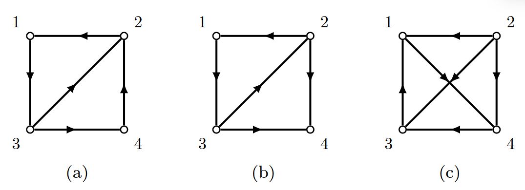
Figure 10 shows several examples of bearing equivalent formations modelled by directed graphs with cycles. As a consequence of the cyclic structure in these graphs, their bearing Laplacians have complex eigenvalues. For some special agents’ positions, the associated bearing Laplacian can have eigenvalues with negative real parts.

• For the example of graph (c) in Figure 10, it can be constructed by adding agent $2$ with three out-going edges to agents 1-3-4 in a cyclic triangle formation (which is bearing equivalent). Therefore, the formation of Figure 10(c) is bearing equivalent according to Proposition 7.
• For all the bearing equivalent formations evaluated in the 2D space in Figure 10, they remain bearing equivalent when agents’ positions are lifted in the 3-D or higher-dimensional space according to the dimensional invariance property in Proposition 8.

A Unified and General Framework [9]

Preliminaries and Notation

• The $d$-sphere, i.e., the unit sphere embedded in ${\mathbb{R}}^{d+1}$, is denoted as ${\mathbb{S}}^d$. We recall that the 1D manifold ${\mathbb{S}}^1$ (corresponding to the unit circle) is isomorphic to the special orthogonal group $\mathrm{SO}(2)=\{\mathbf{R}\in {\mathbb{R}}^{2\times 2}\mid \mathbf{R}{\mathbf{R}}^{\mathrm{\top }}={\mathbf{I}}_2,\det (\mathbf{R})=+1\}$ which can be parametrized by a single angle $\alpha \in [0,2\pi )$.
• The special orthogonal group $\mathrm{SO}(3)=\{\mathbf{R}\in {\mathbb{R}}^{3\times 3}\mid \mathbf{R}{\mathbf{R}}^{\mathrm{\top }}={\mathbf{I}}_3,\det (\mathbf{R})=1\}$, instead, is not isomorphic to the 2 -sphere ${\mathbb{S}}^2$, but it holds that ${\mathbb{S}}^2=\mathrm{SO}(3)/\mathrm{SO}(2)$.
• The Cartesian product ${\mathbb{R}}^d\times \mathrm{SO}(d)$ corresponds to the special Euclidean group $\mathrm{SE}(d)$.

Bearing Rigidity: Definitions and Properties

In this section we introduce the main concepts related to bearing rigidity theory.

Framework Formation Model

Consider a generic formation of $n⩾3$ agents, wherein each agent is associated to an element of the differential manifold ${\mathcal{P}}_i\subseteq \mathrm{SE}(3),i\in \{1,\cdots ,n\}$, describing its configuration and motion constraints.

Here, we focus on real world scenarios, nonetheless the definitions and properties provided in the following are valid also for the case ${\mathcal{P}}_i={\mathbb{R}}^d$ with $d>3$.

In detail, introducing a global frame common (but not necessarily available) to all the agents in the group, the configuration $p_i\in {\mathcal{P}}_i$ of the ith agent coincides with its position when modeled as a particle, or with the pair of its position and (partial/full) attitude, i.e., with its (partial/full) pose, when the rigid body model is assumed. We now introduce the notion of a framework.

Definition: Framework in $\overline{\mathcal{P}}$

A framework embedded in the product differential manifold $\overline{\mathcal{P}}=\prod _{i=1}^n{\mathcal{P}}_i\subseteq \mathrm{SE}(3{)}^n$ is an ordered pair $(\mathcal{G},\mathit{p})$ consisting of a (directed or undirected) graph $\mathcal{G}=(\mathcal{V},\mathcal{E})$ with $|\mathcal{V}|=n$, and a map $\chi :\mathcal{V}⟼\overline{\mathcal{P}}$ such that $v_i⟼\chi (v_i):=p_i\in {\mathcal{P}}_i$. We refer to $\mathit{p}=(p_1,\cdots ,p_n)\in \overline{\mathcal{P}}$ as the formation configuration.

The framework model characterizes a formation in terms of the agent configuration, where $\mathit{p}$ can be thought of as an embedding of the graph into $\overline{\mathcal{P}}$, and the agents are associated with nodes in the graph. In the study of bearing rigidity, we are interested in the bearing vector between pairs of agents that are connected by an edge in $\mathcal{G}$. Note that $\mathcal{G}$ can be directed or undirected. In rigidity theory, it is typically assumed that the graph is not time-varying, and we adopt this assumption here. We introduce also the following definitions on formations.

Definition: Noncolinear Formation

An $n$-agent formation modeled as a framework $(\mathcal{G},\mathit{p})$ in $\overline{\mathcal{P}}$ is noncolinear if all agents are in distinct positions and do not lie along the same line in the global frame.

Definition: Homogeneous Formation

An $n$-agent formation modeled as a framework $(\mathcal{G},\mathit{p})$ in $\overline{\mathcal{P}}$ is homogeneous if ${\mathcal{P}}_i=\mathcal{P},\mathrm{\forall }i\in \{1,\cdots ,n\}$, hence $\overline{\mathcal{P}}={\mathcal{P}}^n$. Otherwise, the formation is heterogeneous.

Note that, for a noncolinear homogeneous $n$-agent formation, the $(n\times d)$ matrix describing the agents position in ${\mathbb{R}}^d$ is of rank greater than $1$.

Although the stated assumptions regard the agents state and motion constraints, for a given formation the bearing rigidity properties are related to the bearing vector between neighboring agents. According to the framework model, every edge $e_k=e_{ij}=(v_i,v_j)\in \mathcal{E}(|\mathcal{E}|=m)$ represents a bearing measurement $b_k=b_{ij}$ defined in the differential manifold ${\mathcal{M}}_k\subseteq {\mathbb{S}}^2$ and recovered by the $i$ th agent which is able to sense the $j$ th agent, $i,j\in \{1\dots n\},i\ne j$. The bearing measurements domain can now be expressed as $\overline{\mathcal{M}}=\prod _{k=1}^m{\mathcal{M}}_k\subseteq {\mathbb{S}}^{2m}$. For homogeneous formations, it is $\overline{\mathcal{M}}={\mathcal{M}}^m$ with ${\mathcal{M}}_k=\mathcal{M},\mathrm{\forall }k\in \{1\dots m\}$. The available measurements can be expressed in the global frame or in the local frame in-built with each agent/node (and, thus, defined according to ${\mathcal{P}}_i$ ). However, in both cases, these are related to the framework configuration according to the following definition, where an arbitrary edge labeling is introduced.

Definition: Bearing Function

Given an $n$-agent formation modeled as a framework $(\mathcal{G},\mathit{p})$ in $\overline{\mathcal{P}}$, the bearing function is the map ${\mathit{b}}_{\mathcal{G}}:\overline{\mathcal{P}}\to \overline{\mathcal{M}}$ associating the formation configuration $\mathit{p}\in \overline{\mathcal{P}}$ to the vector ${\mathit{b}}_{\mathcal{G}}(\mathit{p})=[b_1^{\mathrm{\top }}\dots b_m^{\mathrm{\top }}{]}^{\mathrm{\top }}\in \overline{\mathcal{M}}$, stacking all the available bearing measurements.

Observe that the bearing function determines the shape of the formation in terms of relative pose among all the agents. One of the central questions in bearing rigidity theory is if a given formation with its bearing function uniquely defines the shape. This will explored in the sequel.

Hereafter, the framework model is adopted to refer to an nagent formation (implying $n⩾3$) and the two concepts (framework and formation) are assumed to be equivalent.

Rigidity Properties of Static Frameworks

Definition of bearing function allows to introduce the first two notions related to bearing rigidity theory, namely, the equivalence and the congruence of different frameworks.

Definition: Bearing Equivalence

Two frameworks $(\mathcal{G},\mathit{p})$ and $(\mathcal{G},{\mathit{p}}^{\prime })$ are bearing equivalent(BE) if ${\mathit{b}}_{\mathcal{G}}(\mathit{p})={\mathit{b}}_{\mathcal{G}}({\mathit{p}}^{\prime })$.

Definition: Bearing Congruence

Two frameworks $(\mathcal{G},\mathit{p})$ and $(\mathcal{G},{\mathit{p}}^{\prime })$ are bearing congruence(BC) if ${\mathit{b}}_{\mathcal{K}}(\mathit{p})={\mathit{b}}_{\mathcal{K}}({\mathit{p}}^{\prime })$, where $\mathcal{K}$ is the complete graph associated to $\mathcal{G}$.

Accounting for the preimage under the bearing function, the set $\mathcal{Q}(\mathit{p}):={\mathit{b}}_{\mathcal{G}}^{-1}({\mathit{b}}_{\mathcal{G}}(\mathit{p}))\subseteq \overline{\mathcal{P}}$ includes all the formation configurations ${\mathit{p}}^{\prime }\in \overline{\mathcal{P}}$ such that $(\mathcal{G},{\mathit{p}}^{\prime })$ is Bearing Equivalence to $(\mathcal{G},\mathit{p})$, while the set $\mathcal{C}(\mathit{p}):={\mathit{b}}_{\mathcal{K}}^{-1}({\mathit{b}}_{\mathcal{K}}(\mathit{p}))\subseteq \overline{\mathcal{P}}$ contains all the formation configurations ${\mathit{p}}^{\prime }\in \overline{\mathcal{P}}$ such that $(\mathcal{G},{\mathit{p}}^{\prime })$ is bearing congruence to $(\mathcal{G},\mathit{p})$. Trivially, it follows that $\mathcal{C}(\mathit{p})\subseteq \mathcal{Q}(\mathit{p})$.

The definition of these sets allows to introduce the (local and global) property of bearing rigidity.

Definition: Bearing Rigidity in $\overline{\mathcal{P}}$

A framework $(\mathcal{G},\mathit{p})$ is (locally) bearing rigid (BR) in $\overline{\mathcal{P}}$ if there exists a neighborhood $\mathcal{U}(\mathit{p})\subseteq \overline{\mathcal{P}}$ of $\mathit{p}$ such that

$$\mathcal{Q}(\mathit{p})\cap \mathcal{U}(\mathit{p})=\mathcal{C}(\mathit{p})\cap \mathcal{U}(\mathit{p}).$$

Definition: Global Bearing Rigidity in $\overline{\mathcal{P}}$

A framework $(\mathcal{G},\mathit{p})$ is globally bearing rigid (GBR) in $\overline{\mathcal{P}}$ if every framework which is BE to $(\mathcal{G},\mathit{p})$ is also BC to $(\mathcal{G},\mathit{p})$, i.e., $\mathcal{C}(\mathit{p})=\mathcal{Q}(\mathit{p})$.

Proposition 9

A GBR framework $(\mathcal{G},\mathit{p})$ is also BR.

Proof:

For a GBR framework $(\mathcal{G},\mathit{p})$, it holds that $\mathcal{C}(\mathit{p})=\mathcal{Q}(\mathit{p})$. Consequently, condition from definition of bearing rigidity is valid for $\mathcal{U}(\mathit{p})=\overline{\mathcal{P}}$ demonstrating that the framework is BR.

$◻$

Rigidity Properties of Dynamic Frameworks

In real-world scenarios, however, agents are generally able to move with or within a formation, and, thus, to change their configuration. Here, the motion constraints are captured by the configuration space ${\mathcal{P}}_i$ of each agent.

For this reason, in this section we assume to deal with dynamic agent formations, namely formations modeled as frameworks $(\mathcal{G},\mathit{p})$ with fixed sensing graph $\mathcal{G}$ and $\mathit{p}$ subject to a deformation implied by the variation of the single agent configuration. Formally, we consider the motion of an agent along a curve in its configuration space parameterized by a variable $t\in [0,1]$. Thus, we have that $p_i=p_i(t)\in {\mathcal{P}}_i$ and $\mathit{p}=\mathit{p}(t)=\{p_1(t)\dots p_n(t)\}\in \overline{\mathcal{P}}$.

In this context, we introduce the variation ${\delta }_i$ defined in the $i$-th agent variations domain ${\mathcal{I}}_i$, depending on the ith agent motion constraints. In particular, we assume that

$$\frac{\mathrm{d}{p}_i(t)}{\mathrm{d}t}=f_i(p_i(t),{\delta }_i)$$

where $f_i:{\mathcal{P}}_i\times {\mathcal{I}}_i\to {\mathcal{P}}_i$ is a continuous function. Accounting for the whole formation, we can stack all ${\delta }_i$ into a vector $\mathit{\delta }\in \overline{\mathcal{I}}$ where $\overline{\mathcal{I}}=\prod _{i=1}^n{\mathcal{I}}_i$ is the variations domain. Note that, for homogeneous formations, we have ${\mathcal{I}}_i=\mathcal{I}$, and thus $\overline{\mathcal{I}}={\mathcal{I}}^n$. Hereafter, we interpret the variable $t$ as a time variable and $\mathit{\delta }$ as the vector of commands acting on the formation to attain the desired evolution from an initial formation configuration $\mathit{p}(0)$ to a final one $\mathit{p}(1)$.

Given this setup, our aim is to identify the conditions under which a given dynamic formation deforms while maintaining its rigidity features, i.e., preserving the existing bearings among the agents over time. The relation between $\mathit{\delta }$ and the derivative of the bearing function, clarified in the next definition, constitutes the starting point for the study of the formation rigidity properties.

Definition: Bearing Rigidity Matrix

For a given (dynamic) framework $(\mathcal{G},\mathit{p}(t))$, the bearing rigidity matrix is the matrix $R_{\mathcal{B}}(\mathit{p}(t))$ that satisfies the relation

$$\begin{array}{}\text{(10)}& {\dot{\mathit{b}}}_{\mathcal{G}}(\mathit{p}(t))=\frac{\mathrm{d}}{\mathrm{d}t}{\mathit{b}}_{\mathcal{G}}(\mathit{p}(t))=R_{\mathcal{B}}(\mathit{p}(t))\mathit{\delta }.\end{array}$$

Indeed, $R_{\mathcal{B}}(\mathit{p}(t))$ can be interpreted as a Jacobian matrix within a differential geometry perspective, whose dimensions depend on the spaces $\overline{\mathcal{M}}$ and $\overline{\mathcal{I}}$.

Nevertheless, one can observe that the null space of $R_\mathcal{B}(\boldsymbol{p}(t)) $ always identifies all the (first-order) deformations of $\mathit{p}(t)$ that keep the bearing measurements unchanged (${\dot{\mathit{b}}}_{\mathcal{G}}(\mathit{p}(t))=\mathbf{0}$), following from the Taylor series expansion of the bearing function.

From a physical perspective, such variations of $(\mathcal{G},\mathit{p}(t))$ can be interpreted as sets of command inputs to provide to the agents to drive the formation from an initial configuration $\mathit{p}(0)$ to a final one $\mathit{p}(1)$ belonging to the set $\mathcal{Q}(\mathit{p}(0))$ of equivalent formation configurations. Note that the existence of such paths further implies a smooth mapping from $\mathit{p}(0)$ to $\mathit{p}(1)$, and in this sense, $\mathit{\delta }$ can be interpreted as an instantaneous velocity.

Definition: Infinitesimal Variation

For a given (dynamic) framework $(\mathcal{G},\mathit{p}(t))$, a variation $\mathit{\delta }\in \overline{\mathcal{I}}$ is infinitesimal if and only if $\mathit{\delta }\in \mathrm{Null}(R_{\mathcal{B}}(\mathit{p}(t)))$.

It directly results from $(10)$ that an infinitesimal variation preserves the bearing measurements among all interacting agents. For a given $(\mathcal{G},\mathit{p}(t))$, there may be many infinitesimal variations. However, there exist infinitesimal variations that hold for any graph. This follows from the Lemma 6.

In light of Lemma 6, we introduce the notion of trivial variations by considering the infinitesimal variations related to the complete graph $\mathcal{K}$. These ensure the measurements preservation for each pair of nodes in the formation, i.e., the formation shape preservation in terms of relative poses among the agents.

Definition: Trivial Variation

For a given (dynamic) framework $(\mathcal{G},\mathit{p}(t))$, a variation $\mathit{\delta }\in \overline{\mathcal{I}}$ is trivial if and only if $\mathit{\delta }\in \mathrm{Null}(R_{\mathcal{B}}^{\mathcal{K}}(\mathit{p}(t)))$, where $R_{\mathcal{B}}^{\mathcal{K}}(\mathit{p}(t))$ is the bearing rigidity matrix computed for the complete graph $\mathcal{K}$ associated to $\mathcal{G}$.

Lemma 6 is fundamental for the next definition that constitutes a key concept in rigidity theory.

Definition: Infinitesimal Bearing Rigidity in $\overline{\mathcal{D}}$

A (dynamic) framework $(\mathcal{G},\mathit{p}(t))$ is infinitesimally bearing rigid (IBR) in $\overline{\mathcal{D}}$ if $\mathrm{Null}(R_{\mathcal{B}}(\mathit{p}(t)))=\mathrm{Null}(R_{\mathcal{B}}^{\mathcal{K}}(\mathit{p}(t)))$.

Otherwise, it is infinitesimally bearing flexible (IBF).

From a physical point of view, a framework $(\mathcal{G},\mathit{p}(t))$ is IBR if its trivial variations set ${\mathcal{S}}_t:=\mathrm{Null}(R_{\mathcal{B}}^{\mathcal{K}}(\mathit{p}(t)))$ coincides with its infinitesimal variations set ${\mathcal{S}}_i:=\mathrm{Null}(R_{\mathcal{B}}(\mathit{p}(t)))$. A variation in the set ${\mathcal{S}}_i$ (${\mathcal{S}}_t$) induces a deformation of the configuration $\mathit{p}(0)$ into $\mathit{p}(1)$ that is bearing equivalent (congruent) to the initial one, i.e., $\mathit{p}(1)\in \mathcal{C}(\mathit{p}(0))$. Thus, for an IBF framework, there exists at least a variation that deforms the configuration $\mathit{p}(0)$ to $\mathit{p}(1)\in \mathcal{Q}(\mathit{p}(0))\setminus \mathcal{C}(\mathit{p}(0))$.

In the rest of the paper, we limit our analysis to the dynamic framework case, and whenever it is possible, the time dependency is dropped out to simplify the notation.

Unified Rigidity Theory

Unlike many of the existing works on the bearing rigidity that begin their analysis with a statement of the agent configuration space and the rigidity results are then derived, not in generic terms, but explicitly as a function of the chosen configuration space. A consequence of this approach is the need to rederive and redefine rigidity concepts.

In this section, we show that stemming from the general setup given in the last section, we are able to unify the study of bearing rigidity that holds for any $\overline{\mathcal{P}}$ inside $\mathrm{SE}(3{)}^n$.

The main realization is that any agent can be interpreted as a rigid body acting in 3D space with constraints on its motions (i.e., constrained to move on a differential manifold inside $\mathrm{SE}(3{)}^n$).

This approach leads to a general and constructive form for the rigidity matrix and a necessary and sufficient condition relating infinitesimal bearing rigidity to the rank of this matrix.

We consider a formation where each $i$-th agent, $i\in \{1\dots n\}$, is associated to a set of bearing vectors related to its neighbors defined by the graph $\mathcal{G}$. An agent can vary its configuration within ${\mathcal{P}}_i$ consisting of $c_i^t\in \mathbb{N}$ translational DoFs (TDoFs) and $c_i^r\in \mathbb{N}$ rotational DoFs (RDoFs), where $c_i=c_i^t+c_i^r$ is the dimension of the differential manifold ${\mathcal{P}}_i$. In this work we consider ${\mathcal{P}}_i$ in $SE(3)$, so $c_i^t$ and $c_i^r$ are limited in $[0,3]$.

Independently of $c_i$, each agent in the group can be modeled as a rigid body and associated to a local reference frame ${\mathcal{F}}_i$ whose origin $O_i$ coincides with the agent center of mass. At each time instant $t⩾0$, it is thus possible to describe the pose of the agent in the 3D space through the pair $({\mathit{x}}_i(t),{\mathbf{R}}_i(t))\in \mathrm{SE}(3)$, where the vector ${\mathit{x}}_i(t)=[x_i^x(t),x_i^y(t),x_i^z(t){]}^{\mathrm{\top }}\in {\mathbb{R}}^3$ identifies the position of $O_i$ in the global frame ${\mathcal{F}}_W$ and the matrix ${\mathbf{R}}_i(t)\in \mathrm{SO}(3)$ defines the orientation of ${\mathcal{F}}_i$ w.r.t. ${\mathcal{F}}_W$.

In particular, supposing that the (unit) vectors ${\mathbf{e}}_h\in {\mathbb{S}}^2$, $h\in \{1,2,3\}$ identify the axes of the global frame, we assume that ${\mathbf{R}}_i(t)=\mathbf{R}(\{{\theta }_{i,h}(t),{\mathbf{e}}_h{\}}_{h=1}^3)$ meaning that ${\mathbf{R}}_i(t)$ results from the composition of three consecutive rotations, each of them performed around ${\mathbf{e}}_h$ of an angle ${\theta }_{i,h}(t)$, according to a suitable sequence.

This reasoning remains valid for any representation of 3D rotations.

The parameter $c_i$, on the other hand, is intrinsically related to the dimension of $ \mathcal{P}_i$, and ${\mathit{p}}_i$ may not necessarily coincide with the whole pair $({\mathit{x}}_i(t),{\mathbf{R}}_i(t))$. Specifically, when $c_i<6$, the agent can vary its pose in 3D space only partially.

In light of the last section, the described formation can be modeled as a framework in $\overline{\mathcal{P}}\subseteq \mathrm{SE}(3{)}^n$. Under the assumption that agents do not have access to a global frame, $\mathcal{G}$ is a directed graph encoding that bearings are inherently expressed in the local frames and are not necessarily reciprocal between pair of agents.

Hence, the directed edge $e_k=(v_i,v_j)\in \mathcal{E}$ refers to the bearing of the $j$-th agent obtained by the $i$-th agent. This can be expressed in terms of the relative position and orientation of the agents in ${\mathcal{F}}_W$, namely

$$\begin{array}{}\text{(11)}& {\mathit{b}}_k(t)={\mathit{b}}_{ij}(t)={\mathbf{R}}_i^{\mathrm{\top }}(t)s_{ij}(t){\mathit{x}}_{ij}(t)={\mathbf{R}}_i^{\mathrm{\top }}(t){\overline{\mathit{x}}}_{ij}(t),\end{array}$$

where ${\mathit{x}}_{ij}(t)={\mathit{x}}_j(t)-{\mathit{x}}_i(t)\in {\mathbb{R}}^d$ is the relative position vector, and $s_{ij}(t)=\parallel {\mathit{x}}_{ij}(t){\parallel }^{-1}\in \mathbb{R}$ is the inverse of the relative distance between the $i$-th and $j$-th agent.

To treat in a unified way multiple domains, we can consider the embedding of each ${\mathcal{P}}_i$ into the $\mathrm{SE}(3)$ manifold, thus considering the given formation as a framework $(\mathcal{G},\mathit{p}(t))$ in $\mathrm{SE}(3{)}^n$.

Hereafter, a superscript $+$ is used to highlight the vectors defined in the lifted spaces.

Observing $(11)$, we embed $ \bar{\mathcal{M}}$ into ${\mathbb{S}}^{2m}$ and, according to Definition, the bearing function can be expressed as

$$\begin{array}{}\text{(12)}& {\mathit{b}}_{\mathcal{G}}^{+}(\mathit{p}(t))=\mathrm{diag}(s_{ij}(t){\mathbf{R}}_i^{\mathrm{\top }}(t)){\overline{H}}^{\mathrm{\top }}\mathit{x}(t)\in {\mathbb{S}}^{2m},\end{array}$$

where $\mathit{p}(t)=[{\mathit{p}}_1^{\mathrm{\top }}(t)\dots {\mathit{p}}_n^{\mathrm{\top }}(t){]}^{\mathrm{\top }}\in {\mathbb{R}}^{3n}$ stacks all the agent position vectors. Consistently, the variations domain $\mathcal{I}$ can be embedded in ${\mathbb{R}}^{6n}$ and thus the vector $\mathit{\delta }$ can be substituted by

$$\begin{array}{}\text{(13)}& {\mathit{\delta }}^{+}=[{\mathit{\delta }}_p^{\mathrm{\top }},{\mathit{\delta }}_a^{\mathrm{\top }}{]}^{\mathrm{\top }}\in {\mathbb{R}}^{6n},\end{array}$$

where ${\mathit{\delta }}_p\in {\mathbb{R}}^{3n}$ and ${\mathit{\delta }}_a\in {\mathbb{R}}^{3n}$ are defined by padding with zeros the corresponding components of $\mathit{\delta }$ related to the possible variations of the agents position and attitude, respectively.

This allows to introduce the following definition.

Definition: Extended Bearing Rigidity Matrix

For a given framework $(\mathcal{G},\mathit{p}(t))$ embedded in $\mathrm{SE}(3{)}^n$, the extended bearing rigidity matrix is the matrix $R_{\mathcal{G}}^{+}(\mathit{p}(t))\in {\mathbb{R}}^{3m\times 6n}$ that satisfies the relation

$$\begin{array}{}\text{(14)}& {\dot{\mathit{b}}}_{\mathcal{G}}^{+}(\mathit{p}(t))=\frac{\mathrm{d}}{\mathrm{d}t}{\mathit{b}}_{\mathcal{G}}^{+}(\mathit{p}(t))=R_{\mathcal{B}}^{+}(\mathit{p}(t)){\mathit{\delta }}^{+}.\end{array}$$

Note that since ${\mathit{b}}_{\mathcal{G}}^{+}(\mathit{p}(t))$ can be interpreted as the zero-padded version of the vector ${\mathit{b}}_{\mathcal{G}}(\mathit{p}(t))$ in $(11)$, the relation $(14)$ corresponds to $(10)$ when accounting for the embedding of ${\mathcal{P}}_i$ in $\mathrm{SE}(3)$. The consistency between $R_{\mathcal{B}}(\mathit{p}(t))$ and $R_{\mathcal{B}}^{+}(\mathit{p}(t))$ is guaranteed by the emergence of zero rows in the latter. Along the same line, we also observe that $(13)$ induces a partition of $R_{\mathcal{B}}^{+}(\mathit{p}(t))$ into two blocks, distinguishing between the bearing variations due to the variations of the agents position and orientation, as formalized in the next proposition.

Proposition 10

The extended bearing rigidity matrix can be expressed as

$$\begin{array}{}\text{(15)}& R_{\mathcal{B}}^{+}(\mathit{p}(t))=[{\mathbf{D}}_p(t)\mathbf{U}{\overline{\mathbf{E}}}^{\mathrm{\top }},{\mathbf{D}}_a(t)\mathbf{V}{\overline{\mathbf{E}}}_o^{\mathrm{\top }}]\in {\mathbb{R}}^{3m\times 6n},\end{array}$$

where

1. ${\mathbf{D}}_p(t),{\mathbf{D}}_a(t)\in {\mathbb{R}}^{3m\times 3m}$ are derived from the orthogonal projections of relative position and attitude

$$\begin{array}{rl}{\mathbf{D}}_p(t)& =\mathrm{diag}(s_{ij}(t){\mathbf{R}}_i^{\mathrm{\top }}(t)\mathbf{P}({\overline{\mathit{x}}}_{ij}(t))),\\ {\mathbf{D}}_a(t)& =-\mathrm{diag}({\mathbf{R}}_i^{\mathrm{\top }}(t)[{\overline{\mathit{x}}}_{ij}(t){]}_{\times }),\end{array}$$

2. $\mathbf{U}=\mathrm{diag}({\mathbf{U}}_{ij})\in {\mathbb{R}}^{3m\times 3m}$ and $\mathbf{V}=\mathrm{diag}({\mathbf{V}}_{ij})\in {\mathbb{R}}^{3m\times 3m}$ take into account the (time-invariant) matrices ${\mathbf{U}}_{ij},{\mathbf{V}}_{ij}\in {\mathbb{R}}^{3\times 3}$ defining, respectively, the translational directions of the bearing measurement ${\mathit{b}}_{ij}$ and $i$-th and $j$-th agents rotation directions in the 3D space with respect to the $i$-th agent frame;
3. $\overline{\mathbf{H}},{\overline{\mathbf{H}}}_o\in {\mathbb{R}}^{3n\times 3m}$ are derived from the (time-invariant) incidence matrix of the graph $\mathcal{G}$, where ${\overline{\mathbf{H}}}_o={\mathbf{H}}_o\otimes I_d\in {\mathbb{R}}^{dn\times dm}$.

Details of Proof

According to Definition, the extended bearing rigidity matrix $R_{\mathcal{B}}^{+}(\mathit{p}(t))$ has to map the vector ${\mathit{\delta }}^{+}\in {\mathbb{R}}^{6n}$ to the derivative of the bearing function. By applying the product rule to $(12)$, it follows that

$$\begin{array}{}\text{(16)}& \begin{array}{rl}{\dot{\mathit{b}}}_{\mathcal{G}}^{+}(\mathit{p}(t))=& (\frac{\mathrm{d}}{\mathrm{d}t}\mathrm{diag}(s_{ij}(t)))\mathrm{diag}({\mathbf{R}}_i^{\mathrm{\top }}(t)){\overline{\mathbf{E}}}^{\mathrm{\top }}\mathit{x}(t)\\ & +\mathrm{diag}(s_{ij}(t))\left(\frac{\mathrm{d}}{\mathrm{d}t}\mathrm{diag}({\mathbf{R}}_i^{\mathrm{\top }}(t))\right){\overline{\mathbf{E}}}^{\mathrm{\top }}\mathit{x}(t)\\ & +\mathrm{diag}(s_{ij}(t))\mathrm{diag}({\mathbf{R}}_i^{\mathrm{\top }}(t)){\overline{\mathbf{E}}}^{\mathrm{\top }}\frac{\mathrm{d}}{\mathrm{d}t}\mathit{x}(t).\end{array}\end{array}$$

In light of $(13)$, it is possible to distinguish the measurements variations induced by the variations of the agents position ${\mathit{\delta }}_p$ or attitude ${\mathit{\delta }}_a$: the former contribution refers to the $1^{\text{st}}$ and $3^{\text{rd}}$ addendum in $(16)$, while the latter contribution is related to the $2^{\text{nd}}$ one. Accounting for the agents dynamics when embedded in $\mathrm{SE}(3)$, $(16)$ can then be rearranged as

$$\begin{array}{}\text{(17)}& {\dot{\mathit{b}}}_{\mathcal{G}}^{+}(\mathit{p}(t))={\mathbf{D}}_p(t)\mathbf{U}{\overline{\mathbf{E}}}^{\mathrm{\top }}{\mathit{\delta }}_p+{\mathbf{D}}_a(t)\mathbf{V}{\overline{\mathbf{E}}}_o^{\mathrm{\top }}{\mathit{\delta }}_a,\end{array}$$

where $\mathbf{U}{\overline{\mathbf{E}}}^{\mathrm{\top }},\mathbf{V}{\overline{\mathbf{E}}}_o^{\mathrm{\top }}\in {\mathbb{R}}^{3m\times 3n}$ link the bearing measurements variations to the agents variations. In detail, the $1^{\text{st}}$ addendum in $(17)$ includes the product of three matrices: the matrix ${\overline{\mathbf{E}}}^{\mathrm{\top }}$ translates the variations of the agents position into relative positions (which are scaled bearings), the block matrix $\mathbf{U}$ embeds the variation of each bearing in the manifold ${\mathbb{S}}^2$ and, finally, the block matrix ${\mathbf{D}}_p(t)$ accounts for the projection of each bearing ${\mathit{b}}_{ij}$ in the $i$-th agent local frame. An analogous reasoning can be carried out for the $2^{\text{nd}}$ addendum in $(17)$ where ${\mathbf{D}}_a(t)$ acts similarly to ${\mathbf{D}}_p(t)$ since the skew matrix of the relative position vector is an orthogonal matrix.

$◻$

The table below shows particularization of the structure of the extended bearing matrix in $(15)$ for the differential manifolds:

$\mathcal{P}$	${\mathit{x}}_i$	${\mathbf{R}}_i$	${\mathbf{U}}_{ij}$	${\mathbf{V}}_{ij}$
$\mathrm{SE}$ (3)	$\left[\begin{array}{lll}{x}_i^x& x_i^y& x_i^z\end{array}\right]$	$\mathbf{R}\left({\{{\theta }_{i,h}(t),{\mathbf{e}}_h\}}_{h=1}^3\right)$	${\mathbf{I}}_3$	${\mathbf{I}}_3$
${\mathbb{R}}^3\times {\mathbb{S}}^1$ ${\mathbb{R}}^2\times {\mathbb{S}}^1$	${\left[\begin{array}{lll}{x}_i^x& x_i^y& x_i^z\end{array}\right]}^{\mathrm{\top }}$ ${\left[\begin{array}{lll}{x}_i^x& x_i^y& 0\end{array}\right]}^{\mathrm{\top }}$	$\begin{array}{c}\mathbf{R}({\theta }_i(t),\mathbf{v}),\mathbf{v}=\sum _{h=1}^3{v}_h{\mathbf{e}}_h\\ \mathbf{R}({\theta }_i(t),{\mathbf{e}}_3)\end{array}$	$\begin{array}{c}{\mathbf{I}}_3\\ \left[\begin{array}{lll}{\mathbf{e}}_1& {\mathbf{e}}_2& {\mathbf{o}}_3\end{array}\right]\end{array}$	$\begin{array}{rl}& \left[\begin{array}{ll}{\mathbf{0}}_{3\times 2}& \mathbf{v}\end{array}\right]\\ & \left[\begin{array}{ll}{\mathbf{0}}_{3\times 2}& {\mathbf{e}}_3\end{array}\right]\end{array}$
${\mathbb{R}}^3$ ${\mathbb{R}}^2$	${\left[\begin{array}{lll}{x}_i^x& x_i^y& x_i^z\end{array}\right]}^{\mathrm{\top }}$ ${\left[\begin{array}{lll}{x}_i^x& x_i^y& 0\end{array}\right]}^{\mathrm{\top }}$	${\mathbf{I}}_3$ ${\mathbf{I}}_3$	${\mathbf{I}}_3$ $\left[\begin{array}{lll}{\mathbf{e}}_1& {\mathbf{e}}_2& {\mathbf{0}}_3\end{array}\right]$	${\mathbf{0}}_{3\times 3}$ ${\mathbf{0}}_{3\times 3}$

For any framework embedded in $\overline{\mathcal{P}}\subseteq \mathrm{SE}(3{)}^n$, Proposition 10, thus, provides a construction method and a general structure for the bearing rigidity matrix that can be decomposed into a part related to the formation configuration (the matrices ${\mathbf{D}}_p(t)$ and ${\mathbf{D}}_a(t)$), and a part related to the graph (the matrices $\overline{\mathbf{E}}$ and ${\overline{\mathbf{E}}}_o$). While not the focus of this work, this structure may also assist in understanding the combinatorial interpretation of certain rigidity properties. We then observe that the structure of $\mathbf{U}$ and $\mathbf{V}$ induces a level of sparsity in the extended bearing matrix, which may result in the presence of some null columns and null rows.

The embedding of $\overline{\mathcal{D}}$ in $\mathrm{SE}(3{)}^n$ proposed in this section implies two facts.

On one hand, both the infinitesimal and the trivial variations sets can be lifted from $\overline{\mathcal{I}}$ into ${\mathbb{R}}^{6n}$, thus considering the corresponding sets ${\mathcal{S}}_i^{+}$ and ${\mathcal{S}}_t^{+}$ such that $|{\mathcal{S}}_i^{+}|=|{\mathcal{S}}_i|=q_i$ and $ \vert \mathcal{S}_t^+ \vert = \vert \mathcal{S}_t \vert=q_t$. These new sets are related to the null space of the matrices $R_{\mathcal{B}}^{+}(\mathit{p}(t))$ and $R_{\mathcal{B}}^{\mathcal{K}+}(\mathit{p}(t))$. Indeed, we first observe that ${\mathcal{S}}_i^{+}\subset \mathrm{Null}(R_{\mathcal{B}}^{+}(\mathit{p}(t)))$ and $\mathcal{S}t^+ \subset \operatorname{Null}(R^{\mathcal{K}+}\mathcal{B}(\boldsymbol{p}(t))) $ since the extended bearing rigidity matrix can differ from the rigidity matrix because of the emergence of zero columns in correspondence of zero entries of the vector ${\mathit{\delta }}^{+}$. This fact also justify the presence of other vectors in the null space of both $R_{\mathcal{B}}^{+}(\mathit{p}(t))$ and $R_{\mathcal{B}}^{\mathcal{K}+}(\mathit{p}(t))$: these are characterized by zero and non-zero entries in correspondence to non-zero and zero entries of ${\mathit{\delta }}^{+}$. In addition, because $R_{\mathcal{B}}^{\mathcal{K}+}(\mathit{p}(t))$ includes additional rows as compared to $R_{\mathcal{B}}^{+}(\mathit{p}(t))$ while the structure of the two matrices is the same in terms of zero columns, we conclude that $\mathrm{Null}(R_{\mathcal{B}}^{+}(\mathit{p}(t)))={\mathcal{S}}_i^{+}\oplus {\mathcal{S}}_v^{+}$ and $\mathrm{Null}({\mathbf{B}}_{\mathcal{K}}^{+}(\mathit{p}(t)))={\mathcal{S}}_t^{+}\oplus {\mathcal{S}}_v^{+}$. The set ${\mathcal{S}}_v^{+}$, whose cardinality $q_v=|{\mathcal{S}}_v^{+}|$ corresponds to the number of null columns in ${\mathbf{B}}_{\mathcal{G}}^{+}(\mathit{p}(t))$, represents the set of the virtual variations of the evaluated formation and it includes the command inputs inducing variations of the agent configuration that do not affect the bearing measurements but that are also not allowed by the physical constraints on the agents dynamics.

On the other hand, since also the measurements domain $\overline{\mathcal{M}}$ is lifted into ${\mathbb{S}}^{2m}$, $q_m$ null rows may characterize $R_{\mathcal{B}}^{+}(\mathit{p}(t))$ in correspondence to the the zero entries added to the vector ${\mathit{b}}_{\mathcal{G}}(\mathit{p}(t))$ in order to derive ${\mathit{b}}_{\mathcal{G}}(\mathit{p}(t))$.

We finally provide a rank condition on the extended bearing rigidity matrix that guarantees the infinitesimal rigidity of the corresponding framework embedded in any $\overline{\mathcal{P}}$.

Theorem 18

A non-colinear $n$-agent formation modeled as a framework $(\mathcal{G},\mathit{p}(t))$ in an arbitrary differential manifold $\overline{\mathcal{P}}$ is IBR if and only if

$$\mathrm{rank}(R_{\mathcal{B}}^{+}(\mathit{p}(t)))=\mathrm{rank}(R_{\mathcal{B}}^{\mathcal{K}+}(\mathit{p}(t))).$$

Proof:

Because $\mathrm{rank}(R_{\mathcal{B}}^{+})=6n-q_v-q_i$ and $\mathrm{rank}(R_{\mathcal{B}}^{\mathcal{K}+})=6n-q_v-q_t$, it holds that $\mathrm{rank}(R_{\mathcal{B}}^{+}(\mathit{p}(t)))=\mathrm{rank}(R_{\mathcal{B}}^{\mathcal{K}+}(\mathit{p}(t)))$ if and only if $q_i=q_t$. Due to Lemma 6, the last equivalence is guaranteed if and only if $\mathrm{Null}(R_{\mathcal{B}}^{+}(\mathit{p}(t)))=\mathrm{Null}(R_{\mathcal{B}}^{\mathcal{K}+}(\mathit{p}(t)))$, i.e., the framework is IBR.

$◻$

The table below shows the summary of the principal notions related to bearing rigidity theory for the differential manifolds:

$i$-th agent properties				$n$-agent formation properties
$\mathcal{P}$	$p_i$	$\mathcal{M}$	${\mathbf{b}}_{ij}$	$\mathcal{I}$	$\delta$	IBR condition
${\mathbb{R}}^{d}d\in \{2,3\}$	${\mathit{x}}_i\in {\mathbb{R}}^d$ ( $d$ tdofs +0 rdofs)	${\mathbb{S}}^{d-1}$	${\bar{\mathit{x}}}_{ij}$	${\mathbb{R}}^{dn}$	${\mathit{\delta }}_p={\left[\begin{array}{lll}{\dot{\mathit{x}}}_1^{\mathrm{\top }}& \dots & {\dot{\mathit{x}}}_n^{\mathrm{\top }}\end{array}\right]}^{\mathrm{\top }}$	$\mathrm{rank}(R_{\mathcal{B}}^{\mathcal{K}}(\mathit{p}))=dn-d-1$
${\mathbb{R}}^2\times {\mathbb{S}}^1$	${\mathit{x}}_i\in {\mathbb{R}}^2,{\theta }_i\in [0,2\pi )$ (2 tdofs + 1 rdofs)	${\mathbb{S}}^1$	${\mathbf{R}}_i^{\mathrm{\top }}{\bar{\mathit{x}}}_{ij}$	${\mathbb{R}}^{3n}$	$\mathit{\delta }={\left[\begin{array}{ll}{\mathit{\delta }}_p^{\mathrm{\top }}& {\mathit{\delta }}_a\end{array}\right]}^{\mathrm{\top }}$	$\mathrm{rank}(R_{\mathcal{B}}^{\mathcal{K}}(\mathit{p}))=3n-4$
${\mathbb{R}}^3\times {\mathbb{S}}^1$	$\begin{array}{c}{\mathit{x}}_i\in {\mathbb{R}}^3,{\theta }_i\in [0,2\pi )\\ (3\text{ tdofs }+1\text{ rdofs })\end{array}$	${\mathbb{S}}^2$	${\mathbf{R}}_i^{\mathrm{\top }}{\bar{\mathit{x}}}_{ij}$	${\mathbb{R}}^{4n}$	$\mathit{\delta }={\left[\begin{array}{ll}{\mathit{\delta }}_p^{\mathrm{\top }}& {\mathit{\delta }}_a\end{array}\right]}^{\mathrm{\top }}{\mathit{\delta }}_p={\left[\begin{array}{lll}{\dot{\mathit{x}}}_1^{\mathrm{\top }}& \dots & {\dot{\mathit{x}}}_n^{\mathrm{\top }}\end{array}\right]}^{\mathrm{\top }}{\mathit{\delta }}_a={\left[\begin{array}{lll}{\dot{\theta }}_1^{\mathrm{\top }}& \dots & {\dot{\theta }}_n^{\mathrm{\top }}\end{array}\right]}^{\mathrm{\top }}$	$\mathrm{rank}(R_{\mathcal{B}}^{\mathcal{K}}(\mathit{p}))=4n-5$
${\mathbb{R}}^3\times SO(3)$	$\begin{array}{c}{\mathit{x}}_i\in {\mathbb{R}}^3,{\mathbf{R}}_i\in SO(3)\\ \text{ (3 tdofs + 3 rdofs) }\end{array}$	${\mathbb{S}}^2$	${\mathbf{R}}_i^{\mathrm{\top }}{\bar{\mathit{x}}}_{ij}$	${\mathbb{R}}^{6n}$	$\overline{)\begin{array}{ll}\mathit{\delta }={\left[\begin{array}{ll}{\mathit{\delta }}_p^{\mathrm{\top }}& {\mathit{\delta }}_a\end{array}\right]}^{\mathrm{\top }}& {\mathit{\delta }}_p={\left[\begin{array}{lll}{\dot{\mathit{x}}}_1^{\mathrm{\top }}& \cdots & {\dot{\mathit{x}}}_n^{\mathrm{\top }}\end{array}\right]}^{\mathrm{\top }}\\ {\mathit{\delta }}_a={\left[\begin{array}{lll}{\mathit{\omega }}_1^{\mathrm{\top }}& \cdots & {\mathit{\omega }}_n^{\mathrm{\top }}\end{array}\right]}^{\mathrm{\top }}\end{array}}$	$\mathrm{rank}(R_{\mathcal{B}}^{\mathcal{K}}(\mathit{p}))=6n-7$

References

1. Section 2-3 of Formation shape control based on bearing rigidity by Tolga Eren in 2012, where $k$ edges in the paper is replaced by $m$ here.
2. Section 2.2-4 of Using angle of arrival (bearing) information for localization in robot frameworks by Tolga Eren in 2007
3. Sensor and framework topologies of formations with direction, bearing, and angle information between agents by Tolga Eren, ..., Brian D.O. Anderson
4. Section II of Bearing Rigidity and Almost Global Bearing-Only Formation Stabilization by Shiyu Zhao and Daniel Zelazo for the part "arbitary dimensions". Note that the bearing function $F_B(p)$ is replaced by $B_{\mathcal{G}}(\mathit{p})$
5. Part "BEARING RIGIDITY THEORY" in Bearing rigidity theory and its applications for control and estimation of framework systems: life beyond distance rigidity by Shiyu Zhao and Daniel Zelazo.
6. Section 3 of Localizability and distributed protocols for bearing-based framework localization in arbitrary dimensions by Shiyu Zhao and Daniel Zelazo, where the laplacian matrix is represented as $L_{\mathcal{B}}$ rather than $\mathcal{B}$.
7. Section III of Laman graphs are generically bearing rigid in arbitrary dimensions by Shiyu Zhao etc.
8. Characterizing bearing equivalence in directed graphs by Zhiyong Sun, Shiyu Zhao and Daniel Zelazo.
9. A unified dissertation on bearing rigidity theory by Giulia Michieletto, Angelo Cenedese and Daniel Zelazo.

We use "framwork" to replace the "network"; use $\mathit{z}$ to replace $\mathit{e}$.