Basis

Introduction

"The whole is more than the sum of its parts." by Aristotle

Multiple Vehicles [1,2]

For millions of years, nature has presented examples of collective behavior in groups of insects, birds, and fish. This behavior has arisen to permit sophisticated functions of the group that cannot be achieved by individual members.

Collective behavior serves needs such as foraging for food, defense against predators, aggression against prey, and mating. Fish and birds particularly, as part of their group behavior, often display formation-type behavior. In this type of behavior, the relative positions of the fish or birds are preserved, and the formation moves as a cohesive whole.

Nature is inspiring humans to engineer multi-agent systems that mimic this distributed, coordinated behavior. The agents in such engineering systems are not living beings, but machines such as robots, vehicles, and/or mobile sensors. With this inspiration, formations of robots and autonomous or piloted vehicles are being deployed to tackle problems in both the civilian and military spheres, such as bush-fire control, surveillance, and underwater exploration. For various reasons, a formation of vehicles may constitute a more effective sensor than a single vehicle:

1. Some tasks inherently require multiple sensors with known relative positions. For example, in 3D, when distances to an object of interest are measured, to determine the position of that object, at least 4 distance measurements from noncoplanar sensors with known positions are needed to uniquely localize the object, that is, to determine its position.
2. Multiple sensors may have individually differing functionalities, which in aggregate give a new functionality to the sensor formation. For example, a group of UAV may include radio-frequency direction-sensing sensors on some vehicles and optical sensors on others, to allow target localization and target identification by the entire formation.
3. Small, mobile sensors are often less expensive to deploy than a single large sensor.
4. Multiple mobile sensors can cover a region of interest more quickly than a single sensor when the sensing range is too small to allow the whole region to be scanned from one position.

In conclusion, more efficient and complex task execution, robustness when one or more agents fail, scalability, versatility, adaptability, and lower cost.

Formation control and network localization are two fundamental tasks for multiagent systems that enable them to perform complex missions.

Formation Control [1,8]

From a control point of view, tasks are specified at both the level of the whole formation, determining, for example, way points for a path that the center of gravity of the formation is commanded to follow, as well as for the individual agents of the formation, such as maintaining their relative positions, or shifting from one formation shape to another formation shape. Certainly in formations occurring in nature, and commonly in synthetic formations, there is no single master agent exercising control over all other agents. Control tasks in some way are handled on a decentralized basis.

In meeting these objectives, various systems problems arise. The most basic problem is defining practical architectures for control, communications, and sensing. Suitable architectures, however, cannot be defined independently of one another. An overarching requirement is that architectures be scalable. The scalability requirement imposes the need for significant decentralization of information and controller structures. For example, in a formation of birds, no one bird can be expected to watch all of the other birds and compute its own trajectory using even partial knowledge of the trajectories of all of the other birds. Hence the amount of sensing, communication, and control computation by any one agent must be limited.

The goal of formation control is to direct each agent using local information from neighboring agents so that the entire team forms a desired spatial geometric pattern. While the notion of a formation as a geometric pattern has a natural meaning for robotic systems, it may also correspond to more abstract configurations for the system state of a team of agents.

Network Localization [8]

The goal of network localization is to estimate the location of each agent in a network using locally sensed or communicated information from neighboring agents. Network localization is usually the first step that must be completed before a sensor network provides other services, such as positioning mobile robots or monitoring areas of interest.

Graph Rigidity Theory [2]

Graph theory is a natural tool for describing the multi-agent formation shape as well as the inter-agent sensing, communication, and control topology in the decentralized case. This note is based on an important subset of this theory—rigid graph theory—since it naturally ensures that the inter-agent distance constraints of the desired formation are enforced through the graph rigidity. This implicitly ensures that collisions between agents are avoided while acquiring the formation.

We use the concept of graph rigidity as an abstraction of the rigidity of physical structures. In our case, the “vertices” of the “structure” are the agents and the “bars” connecting the vertices are the inter-agent distance constraints imposed by the desired formation. Within this framework, it is convenient to treat each agent as a point.

Preliminary: Graph Theory [4,5]

Please make sure you are familiar with the concept of graph

Consider an undirected graph with $m$ edges and $n$ vertices, denoted by $\mathcal{G}=(\mathcal{V},\mathcal{E})$ with vertex set $\mathcal{V}=\{v_1,\cdots ,v_n\}=\{1,2,\cdots ,n\}$ and edge set $\mathcal{E}\subset \mathcal{V}\times \mathcal{V}$. The neighbor set ${\mathcal{N}}_i$ is defined as ${\mathcal{N}}_i:=\{j\in \mathcal{V}:(i,j)\in \mathcal{E}\}$

Definition: complete graph

A graph $\mathcal{G}$ is said to be complete if every pair of distinct vertices is connected by an edge, i.e., $m=n(n-1)∕2$. A complete graph with n vertices is symbolized by ${\mathcal{K}}_n$

Definition: path

A path is a trail that goes from an origin vertex to a destination vertex by traversing edges of the graph.

Definition: connected

Two vertices $i$ and $j$ are said to be connected if there exists a path between these vertices. A graph is connected if there is a path between every pair of vertices of $\mathcal{G}$.

• the vertex set: the robots (and we may use the word agent interchangeably in the context)
• the edge set: the communication links between different robots

The incidence matrix: $H=\{h_{kj}\}\in {\mathbb{R}}^{m\times n}$, whose entries are defined as (with arbitrary edge orientations)

$$h_{kj}=\{\begin{array}{ll}1,& \text{the }\mathit{\text{k}}\text{-th edge sinks at node }\mathit{\text{j}}\\ -1,& \text{the }\mathit{\text{k}}\text{-th edge leaves at node }\mathit{\text{j}}\\ 0,& \text{otherwise}\end{array}$$

For a connected and undirected graph, one has:

• $\mathrm{rank}(H)=n-1$
• $\mathrm{null}(H)=\mathrm{span}\{{\mathbf{1}}_n\}$.

Define ${\mathbf{H}}_o\in {\mathbb{R}}^{n\times m}$ as:

$$[{\mathbf{H}}_o{]}_{ij}=\{\begin{array}{ll}-1,& \text{if }{e}_k=(v_i,v_j)\in \mathcal{E}\text{ (outgoing edge)}\\ 0,& \text{otherwise}\end{array}.$$

The adjacency matrix: $A(\mathcal{G})$, a symmetric $n\times n$ matrix encoding the vertex adjacency relationships, with entries

$$A_{ij}=\{\begin{array}{ll}1,& \{i,j\}\in \mathcal{E}\\ 0& \text{otherwise}\end{array}$$

• $A_{ij}=A_{ji}$

The Laplacian matrix: $L(\mathcal{G})$:

$$\begin{array}{c}L(\mathcal{G})=H^{\mathrm{\top }}H=\mathrm{diag}(A\mathbf{1})-A\\ L_{ij}=\{\begin{array}{ll}\sum _{j=1}^n{A}_{ij}=|{\mathcal{N}}_i|,& i=j\\ -A_{ij}=-1\text{ or }0,& i\ne j,=-1\text{ if }(i,j)\in \mathcal{E}\end{array}.\end{array}$$

Lemma: Properties of Laplacian matrix

• $L(\mathcal{G})$ is orientation-independent
• $L(\mathcal{G})$ is symmetric and positive semidefinite
• $\sum _{j=1}^n{L}_{ij}=0,i=1,\cdots ,n.$
• If $\mathcal{G}$ is connected, then $L(\mathcal{G})$ has one and only one zero eigenvalue, with $\mathrm{null}(L(\mathcal{G}))=\mathrm{span}\{\mathbf{1}\}$
• $\mathrm{rank}(L(\mathcal{G}))=n-1$ with $0$ being a simple eigenvalue of $L(\mathcal{G})$ if and only if the directed graph $\mathcal{G}$ contains a (directed) spanning tree
• $x^{\mathrm{\top }}Lx=\sum _{\{i,j\}\in \mathcal{E}}{A}_{ij}(x_i-x_j{)}^2$ where $x$ is a column vector

Definition: induced subgraph

For a graph $\mathcal{G}=(\mathcal{V},\mathcal{E})$, let ${\mathcal{V}}^{\prime }$ be a subset of $\mathcal{V}$, then the subgraph of $\mathcal{G}$ induced by ${\mathcal{V}}^{\prime }$ is the graph ${\mathcal{G}}^{\prime }=({\mathcal{V}}^{\prime },{\mathcal{E}}^{\prime })$ where ${\mathcal{E}}^{\prime }$ includes all those edges of $\mathcal{E}$ that are incident on a vertex pair in ${\mathcal{V}}^{\prime }$.

Framework [2]

Definition: Framework

A framework is simply a realization of a graph at given points in Euclidean space. Specifically, if $p_i\in {\mathbb{R}}^d$ is the coordinate of vertex $i$ w.r.t. some fixed coordinate frame, then a framework $\mathcal{F}$ is a pair $(\mathcal{G},\mathit{p})$ where configuration $\mathit{p}=[p_1,\cdots ,p_n]\in {\mathbb{R}}^{dn}$. We will use the notation $\mathcal{F}=(\mathcal{G},\mathit{p})$ to denote that framework $\mathcal{F}$ is composed of graph $\mathcal{G}$ with coordinates $\mathit{p}$.

The importance of a framework is that it can model a physical structure. That is, consider the so-called “bar-and-joint” framework, which is a structure made of rigid bars joined at their ends by universal joints. A bar-and-joint framework can be used to describe a wide range of static and dynamic structures, such as bridges, mechanical linkages, and biological molecules.

In 2D, treat $p_i=[p_{ix},p_{iy}{]}^{\mathrm{\top }}\in {\mathbb{R}}^2,i\in 1,2,\cdots ,n$ as the position of node $i$. The stacked vector $\mathit{p}=[p_1^{\mathrm{\top }},p_2^{\mathrm{\top }},\cdots ,p_n^{\mathrm{\top }}{]}^{\mathrm{\top }}$ represents the position configuration for all the n nodes. By introducing the matrix $\overline{H}:=H\otimes I_2\in {\mathbb{R}}^{2m\times 2n}$, one can construct the edge space as an image of $\overline{H}$ from the position vector $\mathit{p}$:

$$\begin{array}{}\text{(1)}& \mathit{z}=\overline{H}\mathit{p}\end{array}$$

with $z_k=[z_{kx},z_{ky}{]}^{\mathrm{\top }}\in {\mathbb{R}}^2$ being the relative position vector $p_j-p_i$ for the vertex pair defined by the $k$-th edge. In the following, two notations, $z_k$ and $z_{kij}$ will be used interchangeably to denote the $k$-th edge which links agent $i$ and agent $j$.

Introduce:

$$Z(z)=\mathrm{diag}(z_1,z_2,\cdots ,z_m)\in {\mathbb{R}}^{2m\times m}$$

denote block diagonal matrix of the relative position.

The edge function (Specific for distance rigidity function denoted as ${\mathit{d}}_{\mathcal{G}}(\mathit{p})$) $r_{\mathcal{G}}(\mathit{p}):{\mathbb{R}}^{2n}\to {\mathbb{R}}^m$ associated with the framework $(\mathcal{G},\mathit{p})$ is defined as:

$$\begin{array}{}\text{(2)}& r_{\mathcal{G}}(\mathit{p})=[\cdots ,\parallel p_i-p_j{\parallel }^2,\cdots ]=Z(\mathit{z}{)}^{\mathrm{\top }}\mathit{z},(i,j)\in \mathcal{E}.\end{array}$$

where the norm is the standard Euclidean norm, and the $k$-th component in $r_{\mathcal{G}}(p),\parallel p_i-p_j{\parallel }^2$, corresponds to the square length of edge $z_k$.

Rigidity Theory [1,2]

Rigidity Graphs

Characterized by rigid body

Given a bar-and-joint framework, a fundamental question is whether it is rigid or not. By rigidity, we mean the non-deformation of the structure.

Roughly speaking, a formation is rigid if its only smooth motions are those corresponding to translation or rotation of the whole formation

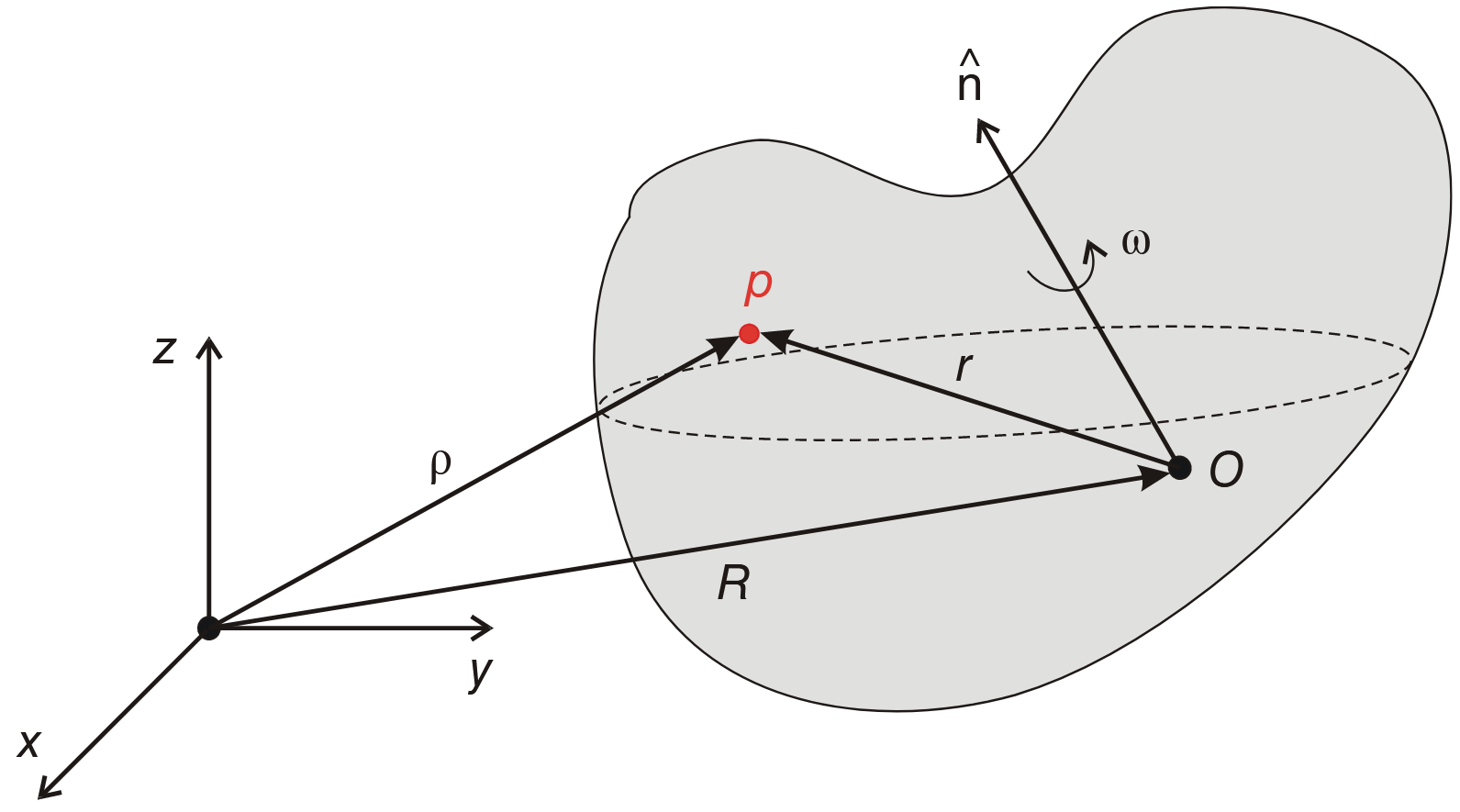
Definition: Translation and Rotation of a rigid body

A rigid body is said to be in translation if all points forming the body move along parallel paths (straight or curvilinear). A rigid body is said to be in rotation if all points move in parallel planes along circles centered on a same axis that intersects the body.

If the axis of rotation does not intersect the rigid body, the motion is usually called a revolution or orbit. This type of motion (in fact, any type of rigid body motion) can be decomposed into a translation superimposed on a rotation. That is, the above definitions allow one to decouple pure translation from pure rotation. Recall from rigid body kinematics that given body-fixed points $p$ and $O$ (see Figure 1.7), the following relationship holds

$$\begin{array}{}\text{(3)}& \dot{\rho }=\dot{R}+\omega \times r\end{array}$$

where $\omega \in {\mathbb{R}}^3$ denotes the angular velocity of the rigid body about an arbitrary axis $\hat{R}$ passing through point $O$ and $\{x,y,z\}$ is an inertial coordinate frame.

Figure 0: Rigid body kinematics.

Definition: Equivalent & Congruent

Two frameworks $(\mathcal{G},\mathit{p})$ and $(\mathcal{G},\hat{\mathit{p}})$ with $\mathcal{G}=(\mathcal{V},\mathcal{E})$ are:

• Equivalent: if $\parallel p_i-p_j\parallel =\parallel {\hat{p}}_i-{\hat{p}}_j\parallel$ for all $(i,j)\in \mathcal{E}$, i.e., the edge function (2) is the same;
• Congruent: if $\parallel p_i-p_j\parallel =\parallel {\hat{p}}_i-{\hat{p}}_j\parallel$ for all $i,j\in \mathcal{V}$ (with $i\ne j$), i.e., all distances between vertices are the same (such $(i,j)$ pairs is always $n(n-1)/2$);

Note that congruency implies equivalency, but the reverse is not necessarily true.

Definition: isometry

An isometry of ${\mathbb{R}}^m$ is a bijective map $T:{\mathbb{R}}^m\to {\mathbb{R}}^m$ such that

$$\parallel T(x)-T(y)\parallel =\parallel x-y\parallel ,\mathrm{\forall }x,y\in {\mathbb{R}}^m.$$

Note that $T$ accounts for rotation and/or translation of the vector $x,y$.

Two frameworks $(\mathcal{G},\mathit{p})$ and $(\mathcal{G},\hat{\mathit{p}})$ are said to be isomorphic in ${\mathbb{R}}^d$ if they are related by an isometry in ${\mathbb{R}}^d$. It is not difficult to see that isomorphic frameworks are congruent. We denote the set of all frameworks that are isomorphic to $\mathcal{F}$ by $\mathrm{Iso}(\mathcal{F})$.

Definition

A motion of a framework $\mathcal{F}=(\mathcal{G},\mathit{p})$ with $\mathcal{G}=(\mathcal{V},\mathcal{E})$ is a continuous family of equivalent frameworks $\mathcal{F}(t)$ for $t\in [0,1]$ where $\mathcal{F}(0)=\mathcal{F}$. That is, each point $p_i,i\in \mathcal{V}$ moves along a continuous trajectory $p_i(t)$ while preserving the distances between points connected by an edge:

$$\begin{array}{}\text{(4)}& \parallel p_i(t)-p_j(t)\parallel =\parallel p_i-p_j\parallel ,(i,j)\in \mathcal{E}.\end{array}$$

This leads us to the following definition of rigidity.

Definition: rigidity

A framework $\mathcal{F}=(\mathcal{G},\mathit{p})$ is rigid in ${\mathbb{R}}^d$ if all of its motions satisfy $p_i(t)=T(p_i),\mathrm{\forall }i\in \mathcal{V}$ , and $\mathrm{\forall }t\in [0,1]$, i.e., the family of frameworks $\mathcal{F}(t)$ is isomorphic.

On the other hand, the framework is flexible in ${\mathbb{R}}^d$ if and only if it is possible to continuously move its vertices to form an equivalent but non-congruent framework.

Chacaterized in Combination

Counting-type conditions related to the graph can be used to ascertain the rigidity or nonrigidity of a generic formation corresponding to the graph.

At first, define the Laman graph.

Definition: Laman Graph

A graph $\mathcal{G}=(\mathcal{V},\mathcal{E})$ is Laman if $|\mathcal{E}|=2|\mathcal{V}|-3$ and every subset of $k⩾2$ vertices spans at most $2k-3$ edges.

The above is a combinatorial definition of Laman graphs. Its intuition is that the edges should be distributed evenly in a Laman graph.

Laman graphs may also be characterized by the Henneberg construction shown in the next 3 sections.

Laman's Theorem

A graph $\mathcal{G}=(\mathcal{V},\mathcal{E})$ modeling a formation in 2D with $n$ vertices and $m$ edges is rigid if and only if there exists a subgraph ${\mathcal{G}}^{\prime }=(\mathcal{V},{\mathcal{E}}^{\prime })$ with $2n-3$ edges such that for every subset ${\mathcal{V}}^{″}$ of $\mathcal{V}$ , the induced subgraph ${\mathcal{G}}^{″}=({\mathcal{V}}^{″},{\mathcal{E}}^{″})$ of ${\mathcal{G}}^{\prime }$ satisfies $|{\mathcal{E}}^{″}|⩽2|{\mathcal{V}}^{″}|-3$.

If a graph $\mathcal{G}=(\mathcal{V},\mathcal{E})$ modeling a formation in 3D of $n$ vertices and $m$ edges is rigid then

• there exists a subgraph ${\mathcal{G}}^{\prime }=(\mathcal{V},{\mathcal{E}}^{\prime })$ with $3n-6$ edges such that, for every subset ${\mathcal{V}}^{″}$ of $\mathcal{V}$ , the induced subgraph ${\mathcal{G}}^{″}=({\mathcal{V}}^{″},{\mathcal{E}}^{″})$ of ${\mathcal{G}}^{\prime }$ satisfies $|\mathcal{E}|⩽3|\mathcal{V}|-6$
• if $|\mathcal{E}|=3|\mathcal{V}|-6$, then $\mathcal{G}$ is 3-connected (equivalently, every pair of vertices of $\mathcal{G}$ is connected by three paths that pairwise have no vertices in common except the end vertices).

Characterized in Linear Algebra

First, embed the graph $\mathcal{G}$ into 2-D space

Definition: (global) rigidity

A framework $(\mathcal{G},p)$ is rigid in ${\mathbb{R}}^2$ if there exists a neighborhood $\mathcal{U}$ of $p$ such that $r_{\mathcal{G}}^{-1}(r_{\mathcal{G}}(p))\cap \mathcal{U}=r_{\mathcal{K}}^{-1}(r_{\mathcal{K}}(p))\cap \mathcal{U}$, where $\mathcal{K}$ is the complete graph with the same vertex set as $\mathcal{G}$.

Two frameworks $(\mathcal{G},\mathit{p})$ and $(\mathcal{G},\overline{\mathit{p}})$ are equivalent if $r_{\mathcal{G}}(\mathit{p})=r_{\mathcal{G}}(\overline{\mathit{p}})$ and are congruent if $\parallel p_i-p_j\parallel =\parallel {\overline{p}}_i-{\overline{p}}_j\parallel$ for all $i,j\in \mathcal{V}$.

Now give the definition of regular point[7].

For a smooth map $f:X\to Y$ where $X$ and $Y$ are smooth manifolds, we denote the derivative of $f$ at $\mathit{x}\in X$ by $\mathrm{d}f(\mathit{x})$. Let $k=max\{\mathrm{rank}(\mathrm{d}f(\mathit{x}))$ : $\mathit{x}\in X\}$. We say that $\mathit{x}\in X$ is a regular point of $f$ if $\mathrm{rank}(\mathrm{d}f(\mathit{x}))=k$ and a singular point otherwise.

Proposition 1

Let $\mathit{f}:{\mathbb{R}}^n\to {\mathbb{R}}^m$ be a smooth map and $k=max\{\mathrm{rank}(\mathrm{d}\mathit{f}(\mathit{x})):\mathit{x}\in {\mathbb{R}}^n\}$. If ${\mathit{x}}_0\in {\mathbb{R}}^n$ is a regular point of $\mathit{f}$, then the image under $\mathit{f}$ of some neighborhood of ${\mathit{x}}_0$ is a $k$-dimensional manifold.

Details of Proof

Let $\mathit{f}=({\mathit{f}}_1,{\mathit{f}}_2)$ where ${\mathit{f}}_1$ consists of the first $k$ coordinate functions of $\mathit{f}$ and assume that $\mathrm{rank}(\mathrm{d}{\mathit{f}}_1({\mathit{x}}_0))=k$. Since $\mathrm{rank}(\mathrm{d}{\mathit{f}}_1)=k$ in a neighborhood of ${\mathit{x}}_0$, the Inverse Function Theorem yields local coordinates at ${\mathit{x}}_0$ such that ${\mathit{f}}_1({\mathit{x}}_1,{\mathit{x}}_2)={\mathit{x}}_1$. Thus in local coordinates

$$\mathrm{d}\mathit{f}=\left[\begin{array}{cc}I& 0\\ \frac{\partial {\mathit{f}}_2}{\partial {\mathit{x}}_1}& \frac{\partial {\mathit{f}}_2}{\partial {\mathit{x}}_2}\end{array}\right]$$

Since $\mathrm{rank}(\mathrm{d}\mathit{f})=k$ near ${\mathit{x}}_0,\partial {\mathit{f}}_2/\partial {\mathit{x}}_2=0$ near ${\mathit{x}}_0$. Hence ${\mathit{f}}_2({\mathit{x}}_1,{\mathit{x}}_2)=g\left({\mathit{x}}_1\right)$ and therefore $\mathit{f}({\mathit{x}}_1,{\mathit{x}}_2)=({\mathit{x}}_1,g\left({\mathit{x}}_1\right))$ near ${\mathit{x}}_0$. Thus $\mathit{f}$ maps some neighborhood of ${\mathit{x}}_0$ onto the graph of $g$ which is a $k$-dimensional manifold.

$◻$

It follows that if $\mathit{p}$ is a regular point of $f_{\mathcal{G}}$, then $f_{\mathcal{G}}^{-1}(f_G(\mathit{p}))$ is a manifold of co-dimension $k$ near $\mathit{p}$. In this case, the construction of a smooth path in non-rigid implies flexible of Proposition 1 is straightforward since near $\mathit{p}$ we then have that $f_{\mathcal{K}}^{-1}(f_{\mathcal{K}}(\mathit{p}))$ is a proper submanifold of $f_{\mathcal{G}}^{-1}(f_{\mathcal{G}}(\mathit{p}))$.

Finally, a subset $M$ of ${\mathbb{R}}^d$ is said to be an affine set if $M$ contains the entire line through each pair of distinct points in $M$. The dimension of an affine set $M$ in ${\mathbb{R}}^d$ is defined to be the dimension of the subspace $M-M=\{x-y:x,y\in M\}$ parallel to $M$ and the affine hull of a set $S\subset {\mathbb{R}}^d$ is the smallest affine set containing $S$. For $\mathit{p}=(p_1,\dots ,p_n)\in {\mathbb{R}}^{dn}$, let $\dim \mathit{p}$ be the dimension of the affine hull of $\{p_1,\dots ,p_n\}$.

Theorem 0

Let $\mathcal{G}$ be a graph with $n$ vertices, $m$ edges, and edge function $f_{\mathcal{G}}$ : ${\mathbb{R}}^{dn}\to {\mathbb{R}}^m$. Suppose that $\mathit{p}\in {\mathbb{R}}^{dn}$ is a regular point of $f_{\mathcal{G}}$. Then the graph $\mathcal{G}(\mathit{p})$ is rigid in ${\mathbb{R}}^d$ if and only if

$$\mathrm{rank}(\mathrm{d}{f}_{\mathcal{G}}(\mathit{p}))=dn-(\dim \mathit{p}+1)(2d-\dim \mathit{p})/2,$$

and $\mathcal{G}(\mathit{p})$ is flexible in ${\mathbb{R}}^d$ if and only if

$$\mathrm{rank}(\mathrm{d}{f}_{\mathcal{G}}(\mathit{p}))<dn-(\dim \mathit{p}+1)(2d-\dim \mathit{p})/2.$$

TODO

Infinitesimal Rigidity

Although our physical intuition can indicate if certain frameworks are rigid or not, in general it is difficult to determine rigidity from the definition characterized by rigid body. Therefore, we will consider a related notion of rigidity called infinitesimal rigidity, which can be easily verified via a matrix rank.

In general, rigidity does not imply infinitesimal rigidity, but infinitesimal rigidity implies rigidity. Frameworks that are rigid but not infinitesimally rigid usually have collinear or parallel edges.

For so-called generic frameworks, rigidity is equivalent to infinitesimal rigidity. When a framework $\mathcal{F}=(\mathcal{G},\mathit{p})$ is generic, then almost all of its realizations have the same rigidity property under small perturbations on $\mathit{p}$. As a result, generic rigidity is a property only of the underlying graph $\mathcal{G}$, i.e., it is independent of almost all $\mathit{p}$. The term “almost all” is used to exclude certain degenerate configurations, such as frameworks that lie in a hyperplane.

For example, The planar framework in Figure below is nongeneric in ${\mathbb{R}}^2$ since vertices $1,2,3,4$ are collinear.

Figure 0.5: A nongeneric framework in 2D real field.

In infinitesimal rigidity, instead of preserving distances during a continuous deformation, we require first-order preservation of distances during an infinitesimal motion. Therefore, infinitesimal rigidity (also called first-order rigidity) is a linear approximation to rigidity.

In the definition of continuous family, i.e. formula $(4)$, the right-hand side is constant by definition. Assuming the trajectories $p_i(t),i\in \mathcal{V}$ are differentiable on $t\in [0,1]$, we square both sides of $(4)$ and differentiate w.r.t. time to obtain

$$\frac{\mathrm{d}}{\mathrm{d}t}\parallel p_i(t)-p_j(t){\parallel }^2=2(p_i(t)-p_j(t){)}^{\mathrm{\top }}({\dot{p}}_i(t)-{\dot{p}}_j(t))=0,(i,j)\in \mathcal{E}.$$

where ${\dot{p}}_i$ denotes the time derivative of $p_i$. Rather than require the formula above be satisfied for all $t\in [0,1]$, we impose the condition that it only need to hold at $t=0$:

$$\begin{array}{}\text{(5)}& (p_i-p_j{)}^{\mathrm{\top }}(v_i-v_j)=0,(i,j)\in \mathcal{E}.\end{array}$$

where $v_i:={\dot{p}}_i(0)$ and $p_i(0)=p_i$ from the definition of continuous family. The above equation leads to a system of $m$ linear equations with the $dn$ unknowns being the velocities $v_i$. When instantaneous velocities $v_i$ that satisfy above formula exist, we say the framework has infinitesimal motion.

Definition: infinitesimal motion [6]

An infinitesimal motion is an assignment of velocities that guarantees the invariance of $r_{\mathcal{G}}(\mathit{p})$, i.e.,

$${\dot{r}}_{\mathcal{G}}(\mathit{p})=\frac{\partial r_{\mathcal{G}}(\mathit{p})}{\partial \mathit{p}}\mathit{v}=0,$$

where $\mathit{v}=({\mathit{v}}_1^{\mathrm{\top }},\cdots ,{\mathit{v}}_n^{\mathrm{\top }}{)}^{\mathrm{\top }},{\mathit{v}}_i={\dot{\mathit{p}}}_i$ is the velocity of vertex $i$. We say a motion is trivial if it satisfies equation above for any framework with $n$ vertices. A framework is infinitesimally rigid if every infinitesimal motion is trivial.

When analyzing infinitesimal rigidity, the rigidity matrix of a framework comes in handy, which is defined as

$$\begin{array}{}\text{(6)}& R_{\mathcal{D}}(\mathit{p})=\frac{1}{2}\frac{\partial r_{\mathcal{G}}(p)}{\partial p}=Z(z{)}^{\mathrm{\top }}\overline{H}\in {\mathbb{R}}^{m\times dn}.\end{array}$$

Note that:

• the entries of $R_{\mathcal{D}}(\mathit{p})$ only involve relative position vectors $z$, and we can rewrite it as $R_{\mathcal{D}}(\mathit{z})$.
• the rigidity matrix has a row for each edge and $2$ columns for each vertex. That is, for the $k$-th edge of $\mathcal{E}$ connecting vertices $i$ and $j$, the $k$-th row of $R$ is $[0,\cdots ,0,(p_i-p_j{)}^{\mathrm{\top }},0,\cdots ,0,(p_j-p_i{)}^{\mathrm{\top }},0,\cdots ,0]$ where $(p_i-p_j{)}^{\mathrm{\top }}$ is in the columns for vertex $i$, $(p_j-p_i{)}^{\mathrm{\top }}$ is in the columns for vertex $j$, and all other elements are zero.

A useful structural property of the rigidity matrix:

$$R_{\mathcal{D}}(\mathit{p})({\mathbf{1}}_n\otimes \mathit{x})=0.$$

given any vector $\mathit{x}\in {\mathbb{R}}^d$.

Using $(6)$, we can conveniently rewrite $(5)$ as

$$\begin{array}{}\text{(7)}& R_{\mathcal{D}}(\mathit{p})\mathit{v}=0\end{array}$$

where $\mathit{v}=[v_1,\cdots ,v_n]\in {\mathbb{R}}^{dn}$. Therefore, infinitesimal motion exists when the above equation has a nontrivial (nonzero) solution $\mathit{v}$. We would like to know when this is the case.

Let $\delta \mathit{p}$ be a variation of $\mathit{p}$. If $R_{\mathcal{D}}(\mathit{p})\delta \mathit{p}=\mathbf{0}$, then $\delta \mathit{p}$ is an infinitesimal (distance) motion of $\mathcal{G}(\mathit{p})$.

Note that if a framework undergoes any rigid body motion, then according to $(3)$ vertex $i$ has velocity

$$v_i=v^{\ast }+\omega \times p_i$$

where $v^{\ast }\in {\mathbb{R}}^3$ is the translational velocity and $\omega \in {\mathbb{R}}^3$ is the angular velocity.

Notice that the vectors are defined here with dimension $3$ irrespective of the Euclidean space of the framework. If the framework is planar, then $v^{\ast }=[v_x^{\ast },v_y^{\ast },0],\omega =[0,0,{\omega }_z],p_i=[p_{ix},p_{iy},0]$.

It is not difficult to check that $(7)$ holds in this case since for the $k$-th row of $R$:

$$\begin{array}{rl}& (p_i-p_j{)}^{\mathrm{\top }}{v}_i+(p_j-p_i{)}^{\mathrm{\top }}{v}_j\\ =& (p_i-p_j{)}^{\mathrm{\top }}(v^{\ast }+\omega \times p_i)+(p_j-p_i{)}^{\mathrm{\top }}(v^{\ast }+\omega \times p_j)\\ =& (p_i-p_j)\cdot (\omega \times p_i)+(p_j-p_i)\cdot (\omega \times p_j)\\ =& p_i\cdot \omega \times p_i-p_j\cdot \omega \times p_i+p_j\cdot \omega \times p_j-p_i\cdot \omega \times p_j\\ =& -p_j\cdot \omega \times p_i-p_i\cdot \omega \times p_j=0\end{array}$$

upon use of the properties of vector products. In other words, rigid body motions produce infinitesimal motions. This leads us to the following definition.

Definition: infinitesimal rigidity

A framework is infinitesimally rigid if the only solutions to $(7)$ arise from rigid body motions. Otherwise, it is infinitesimally flexible.

We can use Definition above to determine if a framework is infinitesimally rigid or flexible by attempting to assign a velocity vector to each vertex such that $(7)$ holds. For example, consider the framework in Figure about nongeneric framework and assign velocity $v_2\in {\mathbb{R}}^2$ to vertex $2$ such that it is any vector perpendicular to $p_1-p_2$ and $p_2-p_3$ while keeping all other velocities at zero, i.e., $\mathit{v}=[0,v_2,0,0,0,0]$. It is easy to see that $R_{\mathcal{D}}(\mathit{p})\mathit{v}=0$ in this case although $\mathit{v}$ is not due to a rigid body motion. Therefore, the framework is infinitesimally flexible. (This framework is, however, rigid since it is nongeneric) This trial-and-error method becomes cumbersome as the complexity of the framework increases or when the framework is generic. More important, it cannot be easily implemented computationally.

Fortunately, there is an easy way of checking whether a framework is infinitesimally rigid via the rank of the rigidity matrix. Before presenting this useful result, we need the following facts:

1. the rank of an $d\times n$ matrix is equal to $n$ minus the dimension of its null space.
2. the number of independent rigid body motions for a generic framework in ${\mathbb{R}}^d$ is $d(d+1)/2$. This means that there exist $3$ independent rigid body motions in ${\mathbb{R}}^2$ (translation along $x$, translation along $y$, and rotation about $z$) and $6$ in ${\mathbb{R}}^3$ (translations along $x,y,z$ and rotations about $x,y,z$).

Given the above, we deduce that $\dim (\mathrm{Null}(R_{\mathcal{D}}(\mathit{p})))⩾d(d+1)/2$ and therefore $\mathrm{rank}(R_{\mathcal{D}}(\mathit{p}))⩽nd-d(d+1)/2$. From Definition of infinitesimal rigidity, we know that for infinitesimally rigid frameworks $\dim (\mathrm{Null}(R_{\mathcal{D}}(\mathit{p})))=d(d+1)/2$ , which gives us the following theorem

Theorem 1 [3]

Consider a framework $(\mathcal{G},p)$ in $d$-dimensional space with $n⩾d$ vertices and $m$ edges. It is infinitesimally rigid if and only if

$$\begin{array}{}\text{(5)}& \mathrm{rank}(R_{\mathcal{D}}(\mathit{p}))=\{\begin{array}{ll}dn-d(d+1)/2,& n⩾d,\\ n(n-1)/2,& n<d\end{array}.\end{array}$$

• $d=2:2n-3$
• $d=3:3n-6$

Obviously, in order to have an infinitesimally rigid framework, the graph should have at least $2n-3$ (resp. $3n-6$) edges in ${\mathbb{R}}^2$ (resp. ${\mathbb{R}}^3$).

From Theorem 1, one knows that the dimension of the null space of $R_{\mathcal{D}}(\mathit{p})$ for an infinitesimally rigid framework $(\mathcal{G},\mathit{p})$ in the $d$-dimensional space is $d(d+1)/2$. The following Lemma characterizes the structure of its null space.

Lemma 1: Null space of the rigidity matrix

Suppose the framework $(\mathcal{G},p)$ is infinitesimally rigid with the associated rigidity matrix denoted as $R_{\mathcal{D}}(\mathit{p})$.

• $d=2$: The null space of $R_{\mathcal{D}}(\mathit{p})$ is of dimension $3$ and is described as $\mathrm{null}(R_{\mathcal{D}}(\mathit{p}))=\mathrm{span}(q_1,q_2,q_3)$, where

$$\begin{array}{c}{q}_1={\mathbf{1}}_n\otimes \left[\begin{array}{c}1\\ 0\end{array}\right],q_2={\mathbf{1}}_n\otimes \left[\begin{array}{c}0\\ 1\end{array}\right]\\ q_3=[(K_3{p}_1{)}^{\mathrm{\top }},(K_3{p}_2{)}^{\mathrm{\top }},\cdots ,(K_3{p}_n{)}^{\mathrm{\top }}{]}^{\mathrm{\top }}\end{array}$$

and the matrix $K_3$ is defined as

$$K_3=\left[\begin{array}{cc}0& 1\\ -1& 0\end{array}\right]$$

• $d=3$: The null space of $R_{\mathcal{D}}(\mathit{p})$ is of dimension $6$ and is described as $\mathrm{null}(R_{\mathcal{D}}(\mathit{p}))=\mathrm{span}(q_1,q_2,q_3,q_4,q_5,q_6)$, where

$$\begin{array}{c}{q}_1={\mathbf{1}}_n\otimes \left[\begin{array}{c}1\\ 0\\ 0\end{array}\right],q_2={\mathbf{1}}_n\otimes \left[\begin{array}{c}0\\ 1\\ 0\end{array}\right]q_3={\mathbf{1}}_n\otimes \left[\begin{array}{c}0\\ 0\\ 1\end{array}\right]\\ q_i=[(K_i{p}_1{)}^{\mathrm{\top }},(K_i{p}_2{)}^{\mathrm{\top }},\cdots ,(K_i{p}_n{)}^{\mathrm{\top }}{]}^{\mathrm{\top }},i=4,5,6\end{array}$$

and the matrix $K_i$ is defined as

$$K_4=\left[\begin{array}{ccc}0& 0& 0\\ 0& 0& -1\\ 0& 1& 0\end{array}\right],K_5=\left[\begin{array}{ccc}0& 0& 1\\ 0& 0& 0\\ -1& 0& 0\end{array}\right],K_6=\left[\begin{array}{ccc}0& -1& 0\\ 1& 0& 0\\ 0& 0& 0\end{array}\right]$$

TODO Proof

Lemma 2

Suppose the framework $(\mathcal{G},\mathit{p})$ is infinitesimally rigid. Then for any node $i$, the set of relative position vectors $p_j-p_i,j\in {\mathcal{N}}_i$ cannot all be collinear (in the 2-D case) or all be coplanar (in the 3-D case).

TODO Proof

• if $(\mathcal{G},\mathit{p})$ is infinitesimally rigid, so is $(\mathcal{G},{\mathit{p}}^{\prime })$ for a generic (open and dense) set of ${\mathit{p}}^{\prime }$.
• Generally speaking, infinitesimal rigidity implies rigidity, but the converse is not true.

As discussed earlier, the rigidity property of a generic framework $\mathcal{F}=(\mathcal{G},\mathit{p})$ is invariant under small perturbations on $\mathit{p}$. With the intent of formalizing this idea, we introduce the following result.

Theorem 2

Consider two frameworks $\mathcal{F}=(\mathcal{G},\mathit{p})$ and $\overline{\mathcal{F}}=(\mathcal{G},\overline{\mathit{p}})$ sharing the same graph. If $\mathcal{F}$ is infinitesimally rigid and $\mathrm{dist}(\overline{\mathit{p}},\mathrm{Iso}(\mathcal{F}))⩽\epsilon$ where $\epsilon$ is a sufficiently small positive constant, then $\overline{\mathcal{F}}$ is also infinitesimally rigid.

Here,

$$\mathrm{dist}(\overline{\mathit{p}},\mathrm{Iso}(\mathcal{F})):=\underset{\mathit{x}\in \mathrm{Iso}(\mathcal{F})}{inf}\parallel \overline{\mathit{p}}-\mathit{x}\parallel .$$

Details of Proof

Let $\hat{\mathcal{F}}=(\mathcal{G},\hat{\mathit{p}})\in \mathrm{Iso}(\mathcal{F})$ be such that

$$\mathrm{dist}(\overline{\mathit{p}},\mathrm{Iso}(\mathcal{F}))=\underset{\mathit{x}\in \mathrm{Iso}(\mathcal{F})}{inf}\parallel \overline{\mathit{p}}-\mathit{x}\parallel =\parallel \overline{\mathit{p}}-\hat{\mathit{p}}\parallel .$$

Obviously, $\hat{\mathcal{F}}$ is infinitesimally rigid since it is isomorphic to $\mathcal{F}$. Therefore, $\mathrm{rank}(R_{\mathcal{D}}(\hat{\mathit{p}}))=2n-3$ according to Theorem 1, and there exists a $(2n-3)\times (2n-3)$ submatrix of $R_{\mathcal{D}}(\hat{\mathit{p}})$, $R_s(\hat{\mathit{p}})$, such that $det[R_s(\hat{\mathit{p}})]\ne 0$. The submatrix $R_s(\hat{\mathit{p}})$ has nonzero elements of the form $({\hat{p}}_i-{\hat{p}}_j{)}^{\mathrm{\top }},(i,j)\in \mathcal{E}$. Since $\mathrm{dist}(\overline{\mathit{p}},\mathrm{Iso}(\mathcal{F}))=\parallel \overline{\mathit{p}}-\hat{\mathit{p}}\parallel ⩽\epsilon$, it is not difficult to show that $[{\overline{p}}_i{]}_k=[{\hat{p}}_i{]}_k+{\gamma }_{ik}$ where ${\gamma }_{ik}$ is a sufficiently small positive constant. Thus, the nonzero elements of $R_s(\hat{\mathit{p}})$ have the form $[{\overline{p}}_i{]}_k-[{\overline{p}}_j{]}_k=[{\hat{p}}_i{]}_k-[{\hat{p}}_j{]}_k+{\gamma }_{ik}-{\gamma }_{jk}$, which are continuously dependent on $\hat{\mathit{p}}$. Since the eigenvalues of a matrix depend continuously on its elements, and the determinant of a matrix is the product of its eigenvalues, it follows that the determinant continuously depends on the elements of the matrix. Thus, for sufficiently small ${\gamma }_{ik}$, we have that $det[R_s(\hat{\mathit{p}})]\ne 0$ and $\mathrm{rank}(R_s(\overline{\mathit{p}}))=\mathrm{rank}(R_s(\hat{\mathit{p}}))=2n-3$. Now, since $R_s(\overline{\mathit{p}})$ is a full rank submatrix of $R_{\mathcal{D}}(\overline{\mathit{p}})$, we know $\mathrm{rank}(R_{\mathcal{D}}(\overline{\mathit{p}}))=2n-3$, so $\overline{\mathcal{F}}$ is infinitesimally rigid.

$◻$

Minimal Rigidity

It is obvious that adding edges to a graph does not destroy rigidity. A natural question is then: What is the minimum number of edges that ensures rigidity? This is important in practice because it ensures that a formation of multiple agents is rigid with the minimum number of sensing and communication links. The disadvantage of minimal rigidity is that it lacks robustness to the loss of a sensor or communication link since redundant edges are removed from the graph

Definition: minimally rigidity

A formation is minimally rigid if it is rigid and if no single interagent distance constraint can be removed without causing the formation to lose rigidity

A graph is minimally rigid if almost all formations to which the graph corresponds are minimally rigid.

As for minimal rigidity, it can be described in 2D and 3D with the rigidity matrix, is characterizable in 2D with Laman’s theorem, and, in 3D, is the subject of necessary conditions and distinct sufficiency conditions on the graph determined by a formation.

Given a graph with edge set $\mathcal{E}$ and vertex set $\mathcal{V}$, which is known to be rigid, it is additionally minimally rigid in 2D or 3D if and only if $|\mathcal{E}|=2|\mathcal{V}|-3$ or $|\mathcal{E}|=3|\mathcal{V}|-6$, respectively, where $|\mathcal{E}|$ and $|\mathcal{V}|$ are the numbers of edges and vertices of the graph.

Theorem 3

A rigid graph is minimally rigid if and only if $m=dn-d(d+1)/2$.

This leads to the following corollary.

Corollary 1

If a framework is infinitesimally and minimally rigid, then its rigidity matrix has full row rank and $R_{\mathcal{D}}(\mathit{p})R_{\mathcal{D}}^{\mathrm{\top }}(\mathit{p})$ is positive definite.

Details of Proof

Given that the rigidity matrix has $m$ rows and $\mathrm{rank}(R_{\mathcal{D}}(\mathit{p}))=dn-d(d+1)/2$ and $m=dn-d(d+1)/2$ for infinitesimally and minimally rigid frameworks, we know $R_{\mathcal{D}}(\mathit{p})$ is full row rank. Now, let $\mathit{y}=R_{\mathcal{D}}^{\mathrm{\top }}(\mathit{p})\mathit{x}$ and

$$V={\mathit{y}}^{\mathrm{\top }}\mathit{y}⩾0.$$

Note that $V$ is positive definite w.r.t. $y$ and positive semi-definite with respect to $x$. Given that $\mathrm{rank}(R_{\mathcal{D}}(\mathit{p}))=\mathrm{rank}(R_{\mathcal{D}}(\mathit{p})R_{\mathcal{D}}^{\mathrm{\top }}(\mathit{p}))$ and $R_{\mathcal{D}}(\mathit{p})$ is full row rank, we know $R_{\mathcal{D}}(\mathit{p})R_{\mathcal{D}}^{\mathrm{\top }}(\mathit{p})$ is invertible and has no zero eigenvalues. Therefore, $V$ is positive definite w.r.t. $x$ and $R_{\mathcal{D}}(\mathit{p})R_{\mathcal{D}}^{\mathrm{\top }}(\mathit{p})$ is a positive definite matrix.

$◻$

For an infinitesimally minimally distance rigid framework, there must exist a vertex associated with fewer than $4$ distance constraints; otherwise, the total number of distance constraints will be at least $2n$ and thus greater than the minimum number $2n-3$.

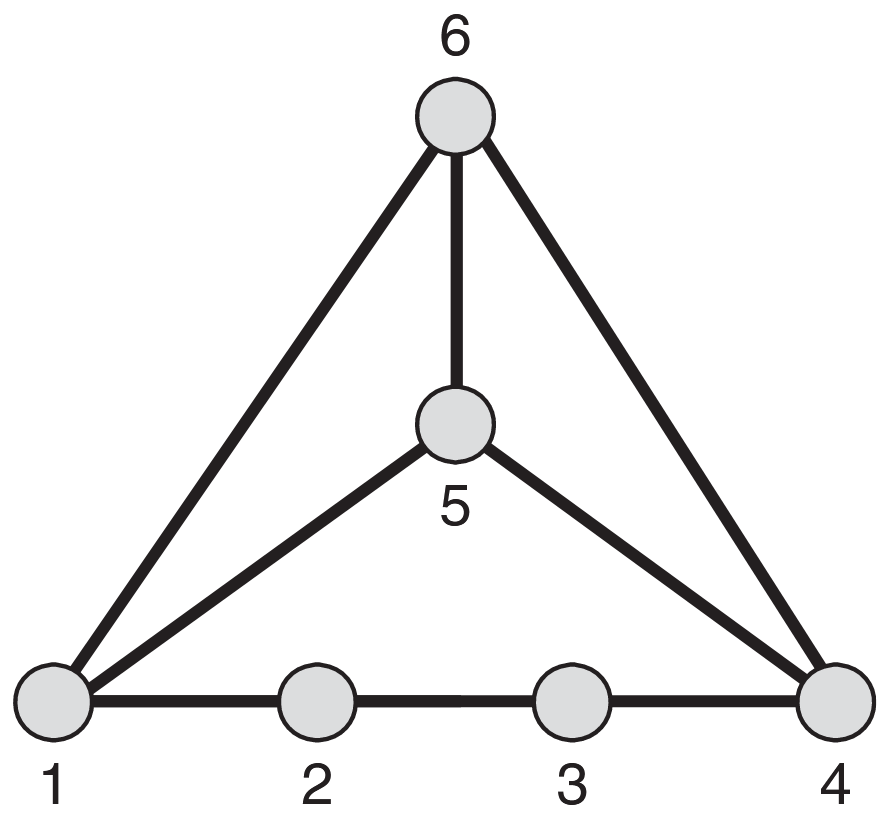
Henneberg construction

The Henneberg construction deals with the iterative construction of rigid formations. As for the characterization of rigidity, the Henneberg construction procedure for 2D formations is better developed than that for 3D formations.

The 2D Henneberg construction comprises the application at each step of one of two possible operations, known as vertex addition and edge splitting.

The procedure begins with a minimally rigid graph, and the application of either operation creates a minimally rigid graph with one additional vertex. Minimally rigid graphs can be progressively built up this way

Definition: Henneberg Construction

The Henneberg construction is a technique for growing minimally rigid graphs, starting from a graph with two vertices and one edge joining the vertices.

At each step in the procedure, illustrated in greater detail below, either a vertex and two edges are added, or a vertex and three new edges are added, while one existing edge is removed. The new edges are incident on the new vertex. These operations are termed vertex addition and edge splitting, respectively.

• vertex addition Let $\mathcal{G}=(\mathcal{V},\mathcal{E})$ be a graph modeling a formation in 2D. A new graph ${\mathcal{G}}^{\prime }=({\mathcal{V}}^{\prime },{\mathcal{E}}^{\prime })$ is formed, where a vertex v is adjoined as well as two edges from $\mathcal{G}$ to $v$ , so that ${\mathcal{V}}^{\prime }=\mathcal{V}\cup \{v\}$ and ${\mathcal{E}}^{\prime }=\mathcal{E}\cup \{(v,j),(v,k)\}$ for some $j,k\in \mathcal{V}$ .

• edge splitting A new graph ${\mathcal{G}}^{\prime }=({\mathcal{V}}^{\prime },{\mathcal{E}}^{\prime })$ is formed from $\mathcal{G}=(\mathcal{V},\mathcal{E})$, where ${\mathcal{V}}^{\prime }=\mathcal{V}\cup \{v\}$ and ${\mathcal{E}}^{\prime }=\mathcal{E}\cup \{(v,j),(v,k),(v,m)\}\mathrm{\setminus }\{e\}$ for some $j,k,m\in \mathcal{V}$ with at least two of the vertices $j,k,m$ adjacent in $\mathcal{G}$, and the edge $e$ either $(j,k),(j,m)$, or $(k,m)$

Figure 1: Growing formations using a Henneberg sequence. (a) The four-agent formation can be expanded to include agent 5 by either (b) a vertex addition operation or (c) an edge-splitting operation. In (b), agent 5 is connected to two distinct agents of the formations. In (c) the edge (1,4) is replaced by two edges (1,5) and (5,4), which are incident on the newly added agent. A third connection (5,2) is also added to the latter agent. Both operations lead to a minimally rigid formation provided that the initial formation is minimally rigid. Moreover, every minimally rigid formation can be obtained by performing a sequence of these operations on an initial formation consisting of two connected agents.

These vertex-addition and edge-splitting operations are enough to grow every minimally rigid graph. It is also possible to deconstruct a minimally rigid graph by removing one vertex and a net count of two edges at each step.

• In growing and deconstructing a minimally rigid graph, all the intermediate graphs are minimally rigid
• A by-product is the fact that every 2D minimally rigid graph is constructible from a primitive comprising a two-vertex single edge graph by using a sequence of these operations
• A Henneberg construction starting from an edge connecting two vertices will result in a Laman graph. The converse is also true. That is if a graph is Laman, then it can be generated by a Henneberg construction

In 3D, operations that are analogous to vertex addition and edge splitting can be defined, but whether these analogously defined operations are necessary and sufficient to build and deconstruct all minimally rigid graphs is still a matter of conjecture

Framework Ambiguities

Consider that a graph $\mathcal{G}=(\mathcal{V},\mathcal{E})$ and the length of each edge (i.e., $\parallel p_i-p_j\parallel ,(i,j)\in \mathcal{E}$) are given. We want to know all frameworks $\mathcal{F}=(\mathcal{G},\mathit{p})$ that are consistent with this data excluding isometries. Can a framework have multiple (non-isomorphic) realizations? There are several sources of nonunique realizations. The trivial one is flexibility, an infinite number of equivalent frameworks exist that satisfy the edge constraints. Infinitesimally rigid frameworks can also suffer from nonuniqueness. Two types of nonuniqueness can occur in this case, but unlike flexibility they lead to a finite number of equivalent frameworks

• flip ambiguity: one vertex can be flip to another side. This occurs when a graph in ${\mathbb{R}}^d$ has a set of vertices lying in a $(d-1)$-dimensional subspace about which a portion of the graph can be reflected. Notice that there cannot be any edges between the portions of the graph separated by the mirror edge.
  • Not every minimally rigid graph contains a flip ambiguity
  • Multiple flips can happen in a given framework
• discontinuous flex ambiguity: positions of 2 or more vertexes can be changed while satisfying the constraints. This occurs in minimally rigid graphs since the removal of an edge allows a portion of the graph to flex. If the removed edge is reinserted after a flexing, one may obtain an equivalent framework with a different configuration.
  • Every formation corresponding to a minimally rigid graph with four or more vertices at generic positions can exhibit flex ambiguity

This leads us to the following definition.

Definition: ambiguous

If two infinitesimally rigid frameworks are equivalent but not congruent, then they are said to be ambiguous.

We denote the set of all ambiguities of an infinitesimally rigid framework $\mathcal{F}$ by $\mathrm{Amb}(\mathcal{F})$. We assume that all frameworks in $\mathrm{Amb}(\mathcal{F})$ are also infinitesimally rigid (This assumption is reasonable and, in fact, holds almost everywhere).

The existence of framework ambiguities is problematic for formation control since the control law cannot distinguish the actual framework from an ambiguous one if only the edge lengths (i.e., inter-agent distances) are being controlled. In such a case, one solution is to initialize the agents sufficiently close to the desired framework to avoid their convergence to an ambiguous framework. From a control theory standpoint, this means that stability results will be local in nature rather than global. The following corollary to Theorem 2 will be helpful in establishing the stability.

Corollary of Theorem 2

Let $\mathcal{F}=(\mathcal{G},\mathit{p})$ and $\overline{\mathcal{F}}=(\mathcal{G},\overline{\mathit{p}})$ be two frameworks sharing the same graph, and consider the function

$$\mathrm{\Psi }(\overline{\mathcal{F}},\mathcal{F})=\sum _{(i,j)\in \mathcal{E}}(\parallel {\overline{p}}_i-{\overline{p}}_j\parallel -\parallel p_i-p_j\parallel {)}^2.$$

If $\mathcal{F}$ is infinitesimally rigid and $\mathrm{\Psi }(\overline{\mathcal{F}},\mathcal{F})⩽\delta$ where $\delta$ is a sufficiently small positive constant, then $\overline{\mathcal{F}}$ is also infinitesimally rigid.

Detail of Proof

First, note that $\mathrm{\Psi }(\overline{\mathcal{F}},\mathcal{F})=0$ implies that $\overline{\mathcal{F}}\in \mathrm{Iso}(\mathcal{F})$ or $\overline{\mathcal{F}}\in \mathrm{Amb}(\mathcal{F})$. Therefore, $\mathrm{\Psi }(\overline{\mathcal{F}},\mathcal{F})⩽\delta$ implies that there is a sufficiently small positive constant $\epsilon$ such that $\mathrm{dist}(\overline{\mathit{p}},\mathrm{Iso}(\mathcal{F}))⩽\epsilon$ or $\mathrm{dist}(\overline{\mathit{p}},\mathrm{Amb}(\mathcal{F}))⩽\epsilon$. From Theorem 2, we know that $\overline{\mathcal{F}}$ is infinitesimally rigid if $\mathrm{dist}(\overline{\mathit{p}},\mathrm{Iso}(\mathcal{F}))⩽\epsilon$. Since the elements of $\mathrm{Amb}(\mathcal{F})$ are infinitesimally rigid, the proof of Theorem 2 can be followed with $\mathrm{Iso}(\mathcal{F})$ replaced by $\mathrm{Amb}(\mathcal{F})$ to show that $\mathrm{dist}(\overline{\mathit{p}},\mathrm{Amb}(\mathcal{F}))⩽\epsilon$ implies $\overline{\mathcal{F}}$ is infinitesimally rigid.

$◻$

Globally Rigidity

Consider a formation with distinctly labeled agents and with some of the interagent distances known. We wish to understand what alternative formation shapes agents can have when they are positioned consistently with the data. Note that if the formation $\mathcal{F}$ is consistent with the data, then so is every rotation, translation, and reflection of $\mathcal{F}$ . However, the existence of alternative formation shapes that are not obtainable from $\mathcal{F}$ through rotation, translation, and reflection is not clear.

Deifnition: globally rigidity

A 2D or 3D formation is globally rigid if and only if one of the following works:

• any two formations corresponding to the distance data differ by a combination of translation, rotation, and reflection
• every framework that is equivalent to $(\mathcal{G},\mathit{p})$ is congruent to $(\mathcal{G},\mathit{p})$
• $r_{\mathcal{G}}^{-1}(r_{\mathcal{G}}(\mathit{p}))=r_{\mathcal{K}}^{-1}(r_{\mathcal{K}}(\mathit{p}))$ shown in the definition of rigidity.

A graph is globally rigid if and only if a generic formation corresponding to the graph is globally rigid.

Global rigidity is a more demanding concept than rigidity since there exist rigid formations that are not globally rigid, and such formations can be converted to globally rigid formations only by the inclusion of additional distance constraints.

• Local rigidity: cannot cannot deform smoothly from one shape. Minimal rigidity therefore allows retention of shape only in the face of potential smooth deformations, although it does not of itself specify what shape is retained. But with same constraints, graph can have different shapes
• Global rigidity: ensure that the shape is unique

Figure 2: Noncongruent rigid formations with the same set of distance constraints. (a) depicts flip ambiguity since vertex A can be flipped over edge (B,C) to the symmetric position A′ while the distance constraints remain the same. (b) depicts discontinuous flex ambiguity since, by temporarily removing edge (A,D), the edge triple (A,E), (A,B), (B,C) can be flexed to obtain positions A′ and B′ such that the edge length (A′,D) equals the edge length (A,D), and thus all of the distance constraints are maintained. The formations (a) and (b) are thus rigid but not globally rigid. Although no smooth motion can deform these formations without affecting the distances between agents connected by edges, the sets of edges and corresponding distance constraints do not uniquely define the relative positions of the agents. In other words, the distance constraints do not specify the formation shape up to a rotation, translation, or reflection.

A nice characterization of global rigidity is available for 2D formations and their associated graphs. No extension is known for 3D formations. The 2D characterization uses the terms redundant rigidity and three connectivity.

Definition: redundant rigidity

An undirected graph is termed redundantly rigid if it remains rigid after the removal of any single edge.

Definition: connected graph

A graph is connected if there is a path from any vertex to any other vertex. A graph is $k$-connected if it remains connected when any $k-1$ vertices are removed. Equivalently, between any two vertices of a $k$-connected graph, there are $k$ paths that have no common edge and no common vertex, except for the end vertices

Theorem 4

A graph $\mathcal{G}=(\mathcal{V},\mathcal{E})$ modeling a formation in 2D of $|\mathcal{V}|$ vertices and $|\mathcal{E}|$ edges is globally rigid if and only if it is redundantly rigid and $3$-connected.

• When a graph is globally rigid, a generic formation corresponding to the graph is also globally rigid.
• A variation of Laman’s theorem is available that characterizes the redundant rigidity property.
• A useful property of a 2D globally rigid formation is that if the positions of 3 noncollinear agents are known, then the positions of all the other agents can be uniquely determined from the interagent distances corresponding to the edges in the formation graph.
• For the trivial case of small graphs $|\text{V}|⩽3$, a complete graph is both necessary and sufficient for global rigidity
• Globally rigid formations with 4 or more agents are not minimally rigid. A reason for using nonminimally rigid formations, where more constraints are imposed than are needed for shape maintenance: loss of a sensor / communication link / control actuator

Application:

• sensor network localization: unit disk graph use the distance data to determine the Euclidean coordinates for the sensor positions that are consistent with the distance set. The Euclidean coordinates, however, become uniquely specified by using further information obtained from designated anchor nodes or sensors, whose positions are known absolutely

Some problems arise in handling nonminimally rigid formations: if the distances between agents in a formation are measured with some noise and controls operate to try to bring certain distances to specified values, a similar type of inconsistency will be likely to arise

Generic Rigidity [8]

One can ask, for a given bar framework $\mathcal{G}(\mathit{p})$, whether it is globally rigid. However, it is shown that this problem is strongly NP hard even for bar frameworks in ${\mathbb{R}}^1$. We will show that there is an algebraic set of configurations, defined by polynomial equations in the coordinates of the configuration, such that when the configuration $\mathit{p}$ is outside that set, $\mathcal{G}(\mathit{p})$ is globally rigid in ${\mathbb{R}}^2$. However, the complexity of that set of configurations appears to be exponential in $n$, the number of points of the configuration.

So, we are led to consider the question of whether “most” configurations $\mathit{p}$ for a given graph $\mathcal{G}$ are globally rigid.

Definition: algebraically dependent, generic

A set $A=({\alpha }_1,\cdots ,{\alpha }_m)$ of distinct real numbers is said to be algebraically dependent if there is a non-zero polynomial $h(x_1,\cdots ,x_m)$ with integer coefficients such that $h=({\alpha }_1,\cdots ,{\alpha }_m)=0$. If $A$ is not algebraically dependent, it is called generic. If a configuration $\mathit{p}=({\mathit{p}}_1,\cdots ,{\mathit{p}}_n)$ in ${\mathbb{R}}^d$ is such that its $dn$ coordinates are generic, we say $\mathit{p}$ is generic.

We raise a possibly more tractable problem. For a given graph $\mathcal{G}$, when $\mathcal{G}(\mathit{p})$ is globally rigid for all generic configurations $\mathit{p}$ in ${\mathbb{R}}^d$ we say that $\mathcal{G}$ itself is generically globally rigid in ${\mathbb{R}}^d$. So for a fixed dimension $d$ we ask whether a given graph $\mathcal{G}$ is generically globally rigid.

For $d=1$, it is easy to see that $\mathcal{G}$ is generically globally rigid if and only if $\mathcal{G}$ is vertex $2$-connected, which means that it takes the removal of at least two vertices of $\mathcal{G}$ to disconnect the rest of the vertices. In general a graph is vertex $m$-connected if it takes the removal of at least $m$ vertices of $\mathcal{G}$ to disconnect the rest of the vertices.

For $d=2$, here we now have complete information about generic global rigidity for any graph. A framework $\mathcal{G}(\mathit{p})$ in ${\mathbb{R}}^d$ is said to be redundantly rigid if $\mathcal{G}(\mathit{p})$ is rigid in ${\mathbb{R}}^d$ even after the removal of any edge of $\mathcal{G}$.

Theorem 5 (Theorem 4 in arbitary dimension)

Let $\mathcal{G}(\mathit{p})$ be a framework in ${\mathbb{R}}^d$ such that the configuration $\mathit{p}$ is generic, and $\mathcal{G}(\mathit{p})$ is globally rigid with at least $d+1$ vertices. Then the following conditions must hold:

1. The graph $\mathcal{G}$ is vertex $(d+1)$-connected.
2. The framework $\mathcal{G}(\mathit{p})$ is redundantly rigid in ${\mathbb{R}}^d$ .

Condition 1 is clear. One just reflects the vertices on one side of a hyperplane through any separating set of $d$ vertices. Condition 2 is more subtle. Roughly the idea is to remove an edge from $\mathcal{G}$, let the resulting framework flex, and replace the edge in a different configuration.

It is natural to conjecture that conditions 1 and 2 are sufficient for generic global rigidity as well as necessary. Unfortunately, for $d⩾3$, that conjecture is shown to be false. For $d=3$, the complete bipartite graph $K(5,5)$ is redundantly rigid, vertex $4$-connected, but there are generic configurations, where the corresponding framework is not globally rigid, and it is the only known example. For $d⩾3$ it is somewhat embarrassing to admit that it is not known whether global rigidity is a generic property. This means that if $\mathcal{G}(\mathit{p})$ is a generically rigid framework in ${\mathbb{R}}^d$, and $\mathit{q}$ is another generic configuration in ${\mathbb{R}}^d$, it is not known, except for $d=1$ or $d=2$, whether $\mathcal{G}(\mathit{q})$ is globally rigid.

On the other hand, it is known that rigidity is a generic property. In other words, if $\mathit{p}$ is a generic configuration in ${\mathbb{R}}^d$ , and $\mathit{q}$ is another generic configuration in ${\mathbb{R}}^d$ , it is known that $\mathcal{G}(\mathit{q})$ is rigid if and only if $\mathcal{G}(\mathit{p})$ is rigid. Thus rigidity in ${\mathbb{R}}^d$ is entirely a combinatorial property of the graph $\mathcal{G}$, although a purely combinatorial polynomial time algorithm to determine generic rigidity is known only for $d=1$ and $d=2$.

References

1. Rigid graph control architectures for autonomous formations by D. O. Anderson etc.;
2. Section 1.1-1.3 of Formation Control of Multi-Agent Systems: A Graph Rigidity Approach by Marcio de Queiroz etc.;
3. Theorem from Conditions for unique graph realizations by Bruce Hendrickson;
4. Preliminaries part of Distributed estimation and control for preserving formation rigidity for mobile robot teams by Zhiyong Sun, ..., D. O. Anderson;
5. Preliminaries part of Distributed stabilization control of rigid formations with prescribed orientation by Zhiyong Sun, ..., D. O. Anderson, Hyo-Sung Ahn
6. Preliminaries part of Angle-based shape determination theory of planar graphs with application to formation stabilization by Gangshan Jing, etc..
7. The Rigidity of Graphs by L. Asimow and B. Roth in 1978.
8. Part 1.2: Generic Global Rigidity in Generic Global Rigidity by Robert Connelly
9. 1st Part in Bearing rigidity theory and its applications for control and estimation of framework systems: life beyond distance rigidity by Shiyu Zhao and Daniel Zelazo.

References

- B. D. O. Anderson, C. Yu, B. Fidan, and J. M. Hendrickx, Rigid graph control architectures for autonomous formations, IEEE Control Syst. Mag., vol. 28, no. 6, pp. 48–63, Dec. 2008.
- Marcio de Queiroz, Xiaoyu Cai, and Matthew Feemster, Formation Control of Multi-Agent Systems: A Graph Rigidity Approach. USA: John Wiley & Sons, Ltd, 2019. Accessed: Dec. 31, 2025: Section 2.
- Bruce Hendrickson, Conditions for unique graph realizations, SIAM J. Comput., vol. 21, no. 1, pp. 65–84, Feb. 1992.
- Zhiyong Sun, Changbin Yu, and B. D. O. Anderson, Distributed estimation and control for preserving formation rigidity for mobile robot teams, Sep. 19, 2013. Accessed: Dec. 29, 2025: Preliminaries part.
- Zhiyong Sun, M.-C. Park, B. D. O. Anderson, and H.-S. Ahn, Distributed stabilization control of rigid formations with prescribed orientation, Automatica J. IFAC, vol. 78, pp. 250–257, Apr. 2017: Preliminaries part.
- Gangshan Jing, G. Zhang, H. W. J. Lee, and L. Wang, Angle-based shape determination theory of planar graphs with application to formation stabilization, Automatica J. IFAC, vol. 105, pp. 117–129, Jul. 2019: Preliminaries part.
- L. Asimow and B. Roth, The Rigidity of Graphs, Transactions of the American Mathematical Society, vol. 245, pp. 279–289, 1978.
- Robert Connelly, Generic Global Rigidity, Discrete Comput. Geom., vol. 33, no. 4, pp. 549–563, Apr. 2005: Part 1.2.
- Shiyu Zhao and Daniel Zelazo, Bearing rigidity theory and its applications for control and estimation of framework systems: life beyond distance rigidity, IEEE Control Syst. Mag., vol. 39, no. 2, pp. 66–83, Apr. 2019: 1st Part.