Skip to content

3 Linear time-Optimal Control ​

3.1 Existence of Time-Optimal Control ​

Consider the linear system of ODE:

{x˙(t)=Mx(t)+Nα(t)x(0)=x0,

for given matrices M∈Mn×n and N∈Mn×m. We'll again take A to be the cube [−1,1]m⊂Rm.

Define next

P[α(⋅)]:=−∫0τ1ds=−τ,

where τ=τ(α(⋅)) denotes the first time the solution of our system hits the origin 0. (If the trajectory never hits 0, we set τ=∞.)

**Optimal Control Problem**

We are given the starting point x0∈Rn, and want to find an optimal control α∗(⋅) s.t.

P[α∗(⋅)]=maxα(⋅)∈AP[α(⋅)].

Then τ∗=−P[α∗(⋅)] is the minimum time to steer to the origin.

Theorem 3.1: Existence of Time-Optimal Control

Let x0∈Rn. Then there exists an optimal bang-bang control α∗(⋅).

Proof: Let τ∗:=inf{t|x0∈C(t)}. We want to show that x0∈C(τ∗); that is, there exists an optimal control α∗(⋅) steering x0 to 0 at time τ∗.

Coose t1≥t2≥t3≥⋯ s.t. x0∈C(tn) and tn→τ∗. Since x0∈C(tn), there exists a control αn(⋅)∈A s.t.

x0=−∫0tnX−1(s)Nαn(s)ds.

If necessary, redefine αn(s) to be 0 for s≥tn. By Alaoglu’s Theorem, there exists a subsequence nk→∞ and a control α∗(⋅) s.t.

αn⇀∗α∗.

We assert that α∗(⋅) is an optimal control. It is easy to check that α∗(s)=0,s≥τ∗. Also

x0=−∫0tnkX−1(s)Nαnk(s)ds=−∫0t1X−1(s)Nαnk(s)ds,

Since αnk=0 for s≥tnk. let nk→∞:

x0=−∫0t1X−1(s)Nα∗(s)ds=−∫0τ∗X−1(s)Nα∗(s)ds

because α∗(s)=0 for s≥τ∗. Hence x0∈C(τ∗), and therefore α∗(⋅) is optimal.

According to Theorem 2.10 there in fact exists an optimal bang-bang control.

◻

3.2 The Maximum Principle for Linear Time-Optimal Control ​

The really interesting practical issue now is understanding how to compute an optimal control α∗(⋅).

Definition

Define K(t,x0) to be the reachable set for time t. That is:

K(t,x0)={x1|there exists α(⋅)∈A which steers from x0 to x1 at time t}.

Since x(⋅) solves ODE, we have x1∈K(t,x0) iff

x1=X(t)x0+X(t)∫0tX−1(s)Nα(s)ds=x(t)

for some control α(⋅)∈A.

Theorem 3.2: Geometry of the set $K$

The set K(t,x0) is convex and closed.

Proof:

  1. (convexity) Let x1,x2∈K(t,x0). Then ∃α1,α2∈A s.t.
x1=X(t)x0+X(t)∫0tX−1(s)Nα1(s)dsx2=X(t)x0+X(t)∫0tX−1(s)Nα2(s)ds,

Let 0≤λ≤1. Then

λx1+(1−λ)x2=X(t)x0+X(t)∫0tX−1(s)N(λα1(s)+(1−λ)α2(s))⏟∈Ads,

and hence λx1+(1−λ)x2∈K(t,x0).

  1. (Closedness) Assume xk∈K(t,x0) for (k=1,2,⋯) and xk→y. We must show y∈K(t,x0). As xk∈K(t,x0). As xk∈K(t,x0),∃αk∈A s.t.
xk=X(t)x0+X(t)∫0tX−1(s)Nαk(s)ds.

According to Alaoglu’s Theorem, there exist a subsequence kj→∞ and α∈A s.t. αk⇀∗α. Let k=kj→∞ in the expression above, to find

y=X(t)x0+X(t)∫0tX−1(s)Nα(s)ds.

Thus y∈K(t,x0), an hence K(t,x0) is closed.

◻

Notation: boundary

If S is a set, we write ∂S to denote the boundary of S.

Recall that τ∗ denotes the minimum time it takes to steer to 0, using the optimal control α∗. Note that then 0∈∂K(τ∗,x0).

Theorem 3.3: Portryagin Maximum Prnciple for Linear Time-Optimal Control

there exists a nonzero vector h s.t.

(M)h⊤X−1(t)Nα∗(t)=maxa∈A{h⊤X−1(t)Na}.

for each time 0≤t≤τ∗.

Interpretation: The significance of this assertion is that if we know h then the maximization principle (M) provides us with a formula for computing α∗(⋅), or at least extracting useful information.

We will see in the next chapter that assertion (M) is a special case of the general Pontryagin Maximum Principle.

Proof:

  1. We know 0∈∂K(τ∗,x0). Since K(τ∗,x0) is convex, There exist a supporting plane to K(τ∗,x0) at 0; this means tat for some g≠0, we have
g⋅x1≤0,∀x1∈K(τ∗,x0).
  1. Now x1∈K(τ∗,x0) iff ∃α(⋅)∈A s.t.
x1=X(τ∗)x0+X(τ∗)∫0τ∗X−1(s)Nα(s)ds.

Also

0=X(τ∗)x0+X(τ∗)∫0τ∗X−1(s)Nα∗(s)ds.

Since g⋅x1≤0, we deduce that

g⊤(X(τ∗)x0+X(τ∗)∫0τ∗X−1(s)Nα(s)ds)≤0=X(τ∗)x0+X(τ∗)∫0τ∗X−1(s)Nα∗(s)ds.

Define h⊤=g⊤X(τ∗). Then

∫0τ∗h⊤X−1(s)Nα(s)ds≤∫0τ∗h⊤X−1(s)Nα∗(s)ds;

and therefore

∫0τ∗h⊤X−1(s)N(α∗−α(s))ds≥0

for all controls α(⋅)∈A.

  1. We claim now that the foregoing implies
h⊤X−1(t)Nα∗(s)=maxa∈A{h⊤X−1(s)Na}

for almost every time s. For suppose not; then there would exists a subset E⊂[0,τ∗] of positive measure, s.t.

h⊤X−1(t)Nα∗(s)<maxa∈A{h⊤X−1(s)Na}

for s∈E. Design a new control α^(⋅) as follows:

(s)^={α∗(s)(s∉E)α(s)(s∈E)

where α(s) is selected s.t.

maxa∈A{h⊤X−1(s)Na}=h⊤X−1(t)Nα(s).

Then

∫Eh⊤X−1(s)N(α∗−α(s))⏟<0ds≥0.

This contradicts Step 2 above.

◻

For later reference, we pause here to rewrite the foregoing into different notation; this will turn out to be a special case of the general theory developed later in Chapter 4. First of all, define the Hamiltonian:

Definition: Hamiltonian

H(x,p,a):=(Mx+Na)⋅p(x,p∈Rn,a∈A).

Theorem 3.4: Another way to write Pontryagin Maximum Principle for Linear Time-Optimal Control

Let α∗(⋅) be a time optimal control and x∗(⋅) the corresponding response.

Then there exists a function p∗(⋅):[0,τ∗]→Rn, s.t.

x˙∗(t)=∇pH(x∗(t),p∗(t),α∗(t)),(ODE)p˙∗(t)=−∇xH(x∗(t),p∗(t),α∗(t)),(ADJ)H(x∗(t),p∗(t),α∗(t))=maxa∈AH(x∗(t),p∗(t),a).(M)

We call (ADJ) the adjoint equations and (M) the maximization principle. The function p∗(⋅) is the costate.

Proof:

  1. Select the vector h as in Theorem 3.3, and consider the system
{p˙∗(t)=−M⊤p∗(t)p∗(0)=h.

The solution is p∗(t)=e−tM⊤h; and hence

p∗(t)⊤=h⊤X−1(t),

Since (e−tM⊤)⊤=e−tM=X−1(t).

  1. We know from condition (M) in Theorem 3.3 that
h⊤X−1(t)Nα∗(t)=maxa∈A{h⊤X−1(t)Na}.

Since p∗(t)⊤=h⊤X−1(t), this means that

p∗(t)⊤(Mx∗(t)+Nα∗(t))=maxa∈A{p∗(t)⊤(Mx∗(t)+Na)}.
  1. Finally, we observe that according to the definition of the Hamiltonian H, the dynamical equations for x∗(⋅),p∗(⋅) take the form (ODE) and (ADJ), as stated in the Theorem.
    ◻

3.3 Examples ​

Example 1: Rocket Railroad Car ​

We recall this example, introduced in §1.2. We have

(ODE)x˙(t)=[0100]⏟Mx(t)+[01]⏟Nα(t)

for

x(t)=(x1(t),x2(t))⊤,A=[−1,1].

According to the Pontryagin Maximum Principle, there exists h≠0 s.t.

h⊤X−1(t)Nα∗(t)=max|a|≤1{h⊤X−1(t)Na}.

We will extract the interesting fact that an optimal control α∗ switches at most one time.

We must compute etM. To do so, we observe:

M0=I,M=[0100]M2=[0100][0100]=0;

and therefore Mk=0 for all k≥2. Consequently,

etM=I+tM=[1t01]

Then

X−1(t)=[1−t01]X−1(t)N=[1−t01][01]=[−t1]h⊤X−1(t)N=(h1,h2)[−t1]=−th1+h2.

The Maximum Principle asserts

(−th1+h2)α∗(t)=max|a|≤1{(−th1+h2)a};

and this implies that

α∗(t)=sgn(−th1+h2)

for the sign function

sgn={1x>00x=0−1x<0

Therefore the optimal control α∗ switches at most once(−th1+h2 is a function of t, i.e. a line); and if h1=0, then α∗ is constant.

Since the optimal control switches at most once, then the control we constructed by a geometric method in §1.3 must have been optimal.

◻

Example 2: Control of a Vibrating Spring ​

Consider next thesimple dynamics

x¨+x=α,

where we interpret the control as an exterior force acting on an oscillating weight (of unit mass) hanging from a spring. Our goal is to design an optimal exterior forcing α∗(⋅) that brings the motion to a stop in minimum time.
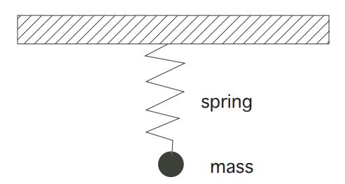
spring model

We have n=2,m=1. The individual dynamical equations read:

{x˙1(t)=x2(t)x˙2(t)=−x1(t)+α(t);

which in vector notation become

x˙(t)=[01−10]⏟Mx(t)+[01]⏟Nα(t)

for |α(t)|≤1. That is, A=[−1,1].

Using the maximum principle ​

We employ the Pontryagin Maximum Principle, which asserts that there exists h≠0 s.t.

(M)h⊤X−1(t)Nα∗(t)=max|a|≤1{h⊤X−1(t)Na}.

To extract useful information from (M) we must compute X(⋅). To do so, we observe that the matrix M is skew symmetric, and thus

M0=I,M=[01−10]M2=[01−10][−100−1]=−I;

Therefore

Mk=Iif k=0,4,8,⋯Mk=Mif k=1,5,9,⋯Mk=−Iif k=2,6,⋯Mk=−Mif k=3,7,⋯

and consequently

etM=I+tM+t22!M2+⋯=I+tM−t22!I−t33!M+t44!I+⋯=(1−t22!+t44!−⋯)I+(t−t33!+t55!−⋯)M=cos⁡tI+sin⁡tM=[cos⁡tsin⁡t−sin⁡tcos⁡t].

So we have

X−1(t)=[cos⁡t−sin⁡tsin⁡tcos⁡t].

and

X−1(t)N=[cos⁡t−sin⁡tsin⁡tcos⁡t][01]=[−sin⁡tcos⁡t]

whence

h⊤X−1(t)N=(h1,h2)[−sin⁡tcos⁡t]=−h1sin⁡t+h2cos⁡t.

According to condition (M), for each time t we have

(−h1sin⁡t+h2cos⁡t)α∗(t)=max|a|≤1{(−h1sin⁡t+h2cos⁡t)a}

Therefore

α∗(t)=sgn(−h1sin⁡t+h2cos⁡t).

Finding the optimal control ​

To simplify further, we may assume h12+h22=1 (unit vector). Recall the trig identity sin⁡(x+y)=sin⁡xcos⁡y+cos⁡xsin⁡y, and choose δ s.t. −h1=cos⁡δ,h2=sin⁡δ. Then

α∗(t)=sgn(cos⁡δsin⁡t+sin⁡δcos⁡t)=sgn(sin⁡(t+δ)).

We deduce therefore that α∗ switches from +1 to −1, and vice versa, every π units of time.

Geometric interpretation ​

Next, we figure out the geometric consequences.

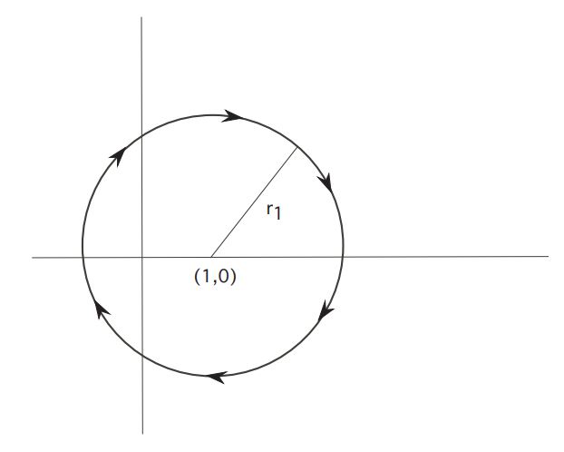
  • When α≡1, our (ODE) becomes

    {x˙1=x2x˙2=−x1+1

    In this case, we can calculate that

    ddt[(x1(t)−1)2+(x2(t))2]=2(x1(t)−1)x˙1(t)+2x2(t)x˙2(t)=2(x1(t)−1)x2(t)+2x2(t)(−x1(t)+1)=0.

    Consequently, the motion satisfies (x1(t)−1)2+(x2(t))2≡r12, for some radius r1, and therefore the trajectory lies on a circle with center (1,0), as illustrated. traj when alpha=1

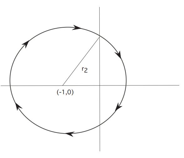
  • If α≡−1, our (ODE) instead becomes

    {x˙1=x2x˙2=−x1−1

    In which case

    ddt[(x1(t)+1)2+(x2(t))2]=0.

    Thus (x1(t)+1)2+(x2(t))2≡r22, for some radius r2, and motion lies on a circle with center (−1,0), as illustrated. traj when alpha=-1

In summary, to get to the origin we must switch our control α(⋅) back and forth between the values ±1, causing the trajectory to switch between lying on circles centered at (±1,0). The switches occur each π units of time.
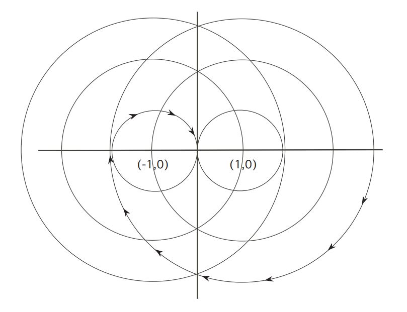
contolled dynamics

Released under the MIT License.