2 Controllablity, bang-bang control

2.1 Definitions

Controllability question

Given the initial point $x^0$ and a “target” set $S\subset {\mathbb{R}}^n$, does there exist a control steering the system to $S$ in finite time?

For the time being we will therefore not introduce any payoff criterion that would characterize an “optimal” control, but instead will focus on the question as to whether or not there exist controls that steer the system to a given goal. In this chapter we will mostly consider the problem of driving the system to the origin $S=\{0\}$.

Definition

Definition: reachable set

• reachable set for time $t$: $\mathcal{C}(t)=$ set of initial points $x^0$ for which there exists a control such that $x(t)=0$

• reachable set: $\mathcal{C}=$ set of initial points $x^0$ for which there exists a control such that $x(t)=0$ for some finite time $t$;

  $$\mathcal{C}=\bigcup _{t\ge 0}\mathcal{C}(t)$$

Let ${\mathbb{M}}^{n\times m}$ denote the set of all $n\times m$ matrices. Assume that this and next chapter, the ODE is linear in both the state $\mathit{x}(\cdot )$ and the control $\mathit{\alpha }(\cdot )$, and he ODE hasthe form

$$\{\begin{array}{l}\dot{\mathit{x}}(t)=M\mathit{x}(t)+N\mathit{\alpha }(t)\\ \mathit{x}(0)=x^0\end{array}$$

where $M\in {\mathbb{M}}^{n\times n}$ and $N\in {\mathbb{M}}^{n\times m}$. Assume the set $A$ of conrol parameters is a cube in ${\mathbb{R}}^m$:

$$A=[-1,1{]}^m=\{a\in {\mathbb{R}}^m||a_i|\le 1,i=1,\dots ,m\}$$

2.2 Quick review of linear ODE

Definition: fundamental solution

Let $\mathit{X}(\cdot ):\mathbb{R}\to {\mathbb{M}}^{n\times n}$ be the unique solution of the matrix ODE:

$$\{\begin{array}{l}\dot{\mathit{X}}(t)=M\mathit{X}(t)(t\in \mathbb{R})\\ \mathit{X}(0)=\mathit{I}.\end{array}$$

We call $\mathit{X}(t)$ the fundamental solution and sometimes write

$$\mathit{X}(t)=e^{tM}:=\sum _{t=0}^{\mathrm{\infty }}\frac{t^k{M}^k}{k!}$$

Last formula being the definition of the exponential $e^{tM}$ and observe that

$${\mathit{X}}^{-1}(t)=\mathit{X}(-t)$$

Theorem 2.1: Solving linear systems of ODE

1. The unique solution of the homogeneous system of ODE$$\{\begin{array}{l}\dot{\mathit{x}}(t)=M\mathit{x}(t)\\ \mathit{x}(0)=x^0.\end{array}$$

is

$$\mathit{x}(t)=\mathit{X}(t)x^0=e^{tM}{x}^0$$

2. The unique solution of the nonhomogeneous system

$$\{\begin{array}{l}\dot{\mathit{x}}(t)=M\mathit{x}(t)+\mathit{f}(t)\\ \mathit{x}(0)=x^0.\end{array}$$

is

$$\mathit{x}(t)=\mathit{X}(t)x^0+\mathit{X}(t){\int }_0^t{\mathit{X}}^{-1}(s)\mathit{f}(s)\mathrm{d}s$$

This expression is the variation of parameters formula.

2.3 Controllability of linear equations

According to the variation of parameters formula, the solution of (linear ODE) for a given control $\mathit{\alpha }(·)$ is

$$\mathit{x}(t)=\mathit{X}(t)x^0+\mathit{X}(t){\int }_0^t{\mathit{X}}^{-1}(s)N\mathit{\alpha }(s)\mathrm{d}s$$$$\begin{array}{rl}& x^0\in \mathcal{C}(t)\\ \leftrightarrow & \text{there exists a control }\mathit{\alpha }(\cdot )\in \mathcal{A}\text{ s.t. }\mathit{x}(t)=0\\ \leftrightarrow & 0=\mathit{X}(t)x^0+\mathit{X}(t){\int }_0^t{\mathit{X}}^{-1}(s)N\mathit{\alpha }(s)\mathrm{d}s\text{ for some control }\mathit{\alpha }(\cdot )\in \mathcal{A}\\ \leftrightarrow & x^0=-{\int }_0^t{\mathit{X}}^{-1}(s)N\mathit{\alpha }(s)\mathrm{d}s\text{ for some control }\mathit{\alpha }(\cdot )\in \mathcal{A}\end{array}$$

Theorem 2.2: Structure of reachable set

1. The reachable set $\mathcal{C}$ is symmetric and convex.
2. Also, if $x^0\in \mathcal{C}(\overline{t})$, then $x^0\in \mathcal{C}(t)$ for all times $t\ge \overline{t}$

Definition

Definition: symmetric & convex

1. A set $S$ is symmetric if $x\in S$ implies $-x\in S$
2. The set $S$ is convex if $x,\hat{x}\in S$ and $0\le \lambda \le 1$ imply $\lambda x+(1-\lambda )\hat{x}\in S$

Proof of theorem 2.2:

1. (Symmetric) Let $t\ge 0$ and $x^0\in \mathcal{C}(t)$. Then $x^0=-{\int }_0^t{\mathit{X}}^{-1}(s)N\mathit{\alpha }(s)\mathrm{d}s$ for some admissible control $\mathit{\alpha }\in \mathcal{A}$.

Therefore $-x^0=-{\int }_0^t{\mathit{X}}^{-1}(s)N(-\mathit{\alpha }(s))\mathrm{d}s$ and $-\mathit{\alpha }(s)\in \mathcal{A}$ since set $A$ is symmetric

Therefore $-x^0\in \mathcal{C}(t)$, and so each set $\mathcal{C}(t)$ symmetric. It follows that $\mathcal{C}$ is symmetric

2. (Convexity) Take $x^0,{\hat{x}}^0\in \mathcal{C}$ so that $x^0\in \mathcal{C},{\hat{x}}^0\in \mathcal{C}(\hat{t})$ for appropriate time $t,\hat{t}\ge 0$. Assume $t\le \hat{t}$. Then

$$\begin{array}{rl}{x}^0& =-{\int }_0^t{\mathit{X}}^{-1}(s)N\mathit{\alpha }(s)\mathrm{d}s\text{ for some control }\mathit{\alpha }(\cdot )\in \mathcal{A}\\ {\hat{x}}^0& =-{\int }_0^{\hat{t}}{\mathit{X}}^{-1}(s)N\hat{\mathit{\alpha }}(s)\mathrm{d}s\text{ for some control }\hat{\mathit{\alpha }}(\cdot )\in \mathcal{A}\end{array}$$

Define a new control

$$\tilde{\mathit{\alpha }}(s):=\{\begin{array}{ll}\mathit{\alpha }(s)& \text{if }0\le s\le t\\ 0& \text{if }s>t\end{array}$$

Then

$$x^0=-{\int }_0^{\hat{t}}{\mathit{X}}^{-1}(s)N\tilde{\mathit{\alpha }}(s)\mathrm{d}s$$

and hence $x^0\in \mathcal{C}(\hat{t})$. Now let $0\le \lambda \le 1$, and observe

$$\lambda x^0+(1-\lambda ){\hat{x}}^0=-{\int }_0^{\hat{t}}{\mathit{X}}^{-1}(s)N(\lambda \tilde{\mathit{\alpha }}(s)+(1-\lambda )\hat{\mathit{\alpha }}(s))\mathrm{d}s$$

Therefore $\lambda x^0+(1-\lambda ){\hat{x}}^0\in \mathcal{C}(\hat{t})\subseteq \mathcal{C}$

3. Assertion (ii) follows from the foregoing if we take $\overline{t}=\hat{t}$.
   $◻$

A simple example

Let $n=2$ and $m=1,A=[-1,1]$, and write $\mathit{x}(t)={(x^1(t),x^2(t))}^T$. Suppose

$$\{\begin{array}{l}{\dot{x}}^1=0\\ {\dot{x}}^2=\alpha (t).\end{array}$$

This is a system of the form $\dot{\mathit{x}}=M\mathit{x}+N\alpha$, for

$$M=\left(\begin{array}{ll}0& 0\\ 0& 0\end{array}\right),N=(\genfrac{}{}{0ex}{}{0}{1})$$

Clearly $\mathcal{C}=\{(x_1,x_2)\mid x_1=0\}$, the $x_2$-axis.

We next wish to establish some general algebraic conditions ensuring that $\mathcal{C}$ contains a neighborhood of the origin

Controllability

Definition: controllability matrix

The controllability matrix is

$$G=G(M,N):=\underset{n\times (mn)\text{ matrix}}{\underbrace{\left[\begin{array}{ccccc}N& MN& M^{2}N& \cdots & M^{n-1}N\end{array}\right]}}$$

Theorem 2.3: Controllability matrix

$$\mathrm{rank}G=n\leftrightarrow 0\in {\mathcal{C}}^{\circ }$$

Notation

• ${\mathcal{C}}^{\circ }$: the interior of the set $\mathcal{C}$, with its own and neighbor fields in the set
• rank of $G$ = number of linearly independent rows / columns of $G$; $\mathrm{rank}G\le n$

Proof:

1. Suppose 1st that $\mathrm{rank}G<n$. This means that the linear span of the columns of G has dimension less than or equal to $n-1$. Thus there exists a vector $b\in {\mathbb{R}}^n,b\ne 0$, orthogonal to each column of $G$. This implies $b^{\mathrm{\top }}G=0$. So

$$b^{\mathrm{\top }}N=b^{\mathrm{\top }}MN=\cdots =b^{\mathrm{\top }}{M}^{n-1}N=0$$

2. In fact, $b^{\mathrm{\top }}{M}^{k}N=0,\mathrm{\forall }k\in {\mathbb{R}}_{+}$ To confirm this, recall that

$$p(\lambda ):=\det (\lambda I-M)$$

is the characteristic polynomial of $M$. The Cayley–Hamilton Theorem states that $p(M)=0$ So if we write

$$p(\lambda )={\lambda }^n+{\beta }_{n-1}{\lambda }^{n-1}+\cdots +{\beta }_1{\lambda }^1+{\beta }_0$$

then

$$p(M)=M^n+{\beta }_{n-1}{M}^{n-1}+\cdots +{\beta }_{1}M+{\beta }_{0}I=0$$

Therefore

$$M^n=-{\beta }_{n-1}{M}^{n-1}-{\beta }_{n-2}{M}^{n-2}-\cdots -{\beta }_{1}M-{\beta }_{0}I$$

and so

$$b^{\mathrm{\top }}{M}^{n}N=b^{\mathrm{\top }}(-{\beta }_{n-1}{M}^{n-1}-\cdots )N=0$$

Similarly, $b^{\mathrm{\top }}{M}^{n+1}N=0$, etc.

Now notice that

$$\begin{array}{rl}{b}^{\mathrm{\top }}{\mathbf{X}}^{-1}(s)N& =b^{\mathrm{\top }}{e}^{-sM}N\\ & =b^T\sum _{k=0}^{\mathrm{\infty }}\frac{(-s{)}^k{M}^{k}N}{k!}\\ & =\sum _{k=0}^{\mathrm{\infty }}\frac{(-s{)}^k}{k!}{b}^T{M}^{k}N=0\end{array}$$

3. Assume next that $x^0\in \mathcal{C}(t)$. This is equivalent to having

$$x^0=-{\int }_0^t{\mathit{X}}^{-1}(s)N\mathit{\alpha }(s)\mathrm{d}s\text{ for some control }\mathit{\alpha }(\cdot )\in \mathcal{A}$$

Then

$$b\cdot x^0=-{\int }_0^t{b}^{\mathrm{\top }}{\mathit{X}}^{-1}(s)N\mathit{\alpha }(s)\mathrm{d}s=0$$

This says that $b$ is orthogonal $x^0$. In other words, $\mathcal{C}$ must lie in the hyperplane orthogonal to $b\ne 0$. Consequently ${\mathcal{C}}^{\circ }=\varphi$.

(How to understand: in the hyperplane, there is no hypersphere in the set)

4. Conversely, assume that $0\notin {\mathcal{C}}^{\circ }$. Thus $0\notin {\mathcal{C}}^{\circ }(t),\mathrm{\forall }t>0$. Since $\mathcal{C}(t)$ is convex, there exits a support hyperplane to $\mathcal{C}(t)$ through $0$(This hyperplane put the set into just one side, and $0$ is not in te interior, so can do this). This means that $\mathrm{\exists }b\ne 0$, s.t. $b\cdot x^0\le 0,\mathrm{\forall }{x}^0\in \mathcal{C}(t)$

(An equation for hyperplane that crosses thre origin is $b\cdot x=0$)

Choose any $x^0\in \mathcal{C}(t)$. Then

$$x^0=-{\int }_0^t{\mathit{X}}^{-1}(s)N\mathit{\alpha }(s)\mathrm{d}s$$

for some control $\mathit{\alpha }$, and therefore

$$0\ge b\cdot x^0=-{\int }_0^t{b}^{\mathrm{\top }}{\mathit{X}}^{-1}(s)N\mathit{\alpha }(s)\mathrm{d}s$$

Thus

$${\int }_0^t{b}^{\mathrm{\top }}{\mathit{X}}^{-1}(s)N\mathit{\alpha }(s)\mathrm{d}s\ge 0\text{ for all controls }\mathit{\alpha }(\cdot )$$

We assert that therefore

$$b^{\mathrm{\top }}{\mathit{X}}^{-1}(s)N\equiv 0$$

a proof of which follows as a lemma below. We rewrite it as

$$b^{\mathrm{\top }}{e}^{-sM}N\equiv 0$$

Let $s=0$ to see that $b^{\mathrm{\top }}N=0$. Next differentiate it with respect to s, to find that

$$b^{\mathrm{\top }}(-M)e^{-sM}N\equiv 0$$

For $s=0$ this says

$$b^{\mathrm{\top }}MN=0$$

We repeatedly differentiate, to deduce

$$b^{\mathrm{\top }}{M}^{k}N=0,\mathrm{\forall }=0,1,\cdots$$

and so $b^{\mathrm{\top }}G=0$. This implies $\mathrm{rank}G<n$, since $b\ne 0$.

$◻$

Lemma 2.4: Integral inequalities

Assume that

$${\int }_0^t{b}^{\mathrm{\top }}{\mathit{X}}^{-1}(s)N\mathit{\alpha }(s)\mathrm{d}s\ge 0$$

for all controls $\mathit{\alpha }(\cdot )$. Then

$$b^{\mathrm{\top }}{\mathit{X}}^{-1}(s)N\equiv 0$$

Proof: Replacing $\mathit{\alpha }$ with $-\mathit{\alpha }$, we see that

$${\int }_0^t{b}^{\mathrm{\top }}{\mathit{X}}^{-1}(s)N\mathit{\alpha }(s)\mathrm{d}s=0$$

for all controls $\mathit{\alpha }(\cdot )$.

Define

$$\mathit{v}(s):=b^{\mathrm{\top }}{\mathit{X}}^{-1}(s)N$$

If $\mathit{v}\ne 0$, then $\mathit{v}(s_0)\ne 0$ for some $s_0$. Then there exists an interval $I$ s.t. $s_0\in I$ and $\mathit{v}(s)\ne 0$ on $I$. Now define $\mathit{\alpha }(\cdot )\in \mathcal{A}$ this way:

$$\{\begin{array}{l}\mathit{\alpha }(s)=0,(s\notin I)\\ \mathit{\alpha }(s)=\frac{\mathit{v}(s)}{|\mathit{v}(s)|}\frac{1}{\sqrt{n}},(s\in I)\end{array}$$

Then

$$0={\int }_0^t\mathit{v}(s)\mathit{\alpha }(s)\mathrm{d}s={\int }_I\frac{\mathit{v}(s)}{\sqrt{n}}\frac{\mathit{v}(s)}{|\mathit{v}(s)|}\mathrm{d}s=\frac{1}{\sqrt{n}}{\int }_I|\mathit{v}(s)|\mathrm{d}s$$

This implies the contradiction that $\mathit{v}\equiv 0$ in $I$.

$◻$

Definition: controllable

We say the linear system (ODE) is controllable if $\mathcal{C}={\mathbb{R}}^n$

Theorem 2.5: Criterion for controllability

Let $A$ be the cube $[-1,1{]}^n$ in ${\mathbb{R}}^n$. Suppose as well that $\mathrm{rank}G=n$, and $\mathrm{Re}\lambda <0$ for each eigenvalue $\lambda$ of the matrix $M$. Then the system(ODE) is controllable

Proof: Since $\mathrm{rank}G=n$, Theroem 2.3 tells us that $\mathcal{C}$ contains some ball $B$ centered at $0$. Now take any $x^0\in {\mathbb{R}}^n$ and consider the evolution

$$\{\begin{array}{l}\dot{\mathit{x}}(t)=M\mathit{x}(t)\\ \mathit{x}(0)=x^0\end{array}$$

in other words, take the control $\mathit{\alpha }(\cdot )\equiv 0$. Since $\mathrm{Re}\lambda <0$ for each eigenvalue $\lambda$ of the matrix $M$, then the origin is asymptotically stable. So ther exists a time $T$ s.t. $\mathit{x}(t)\in B$. Thus $\mathit{x}(T)\in B\subset \mathcal{C}$; and hence there exists a control $\mathit{\alpha }(\cdot )\in \mathcal{A}$ steering $\mathit{x}(t)$ into $0$ in finite time.

$◻$

Example We once again consider the rocket railroad car, from §1.2, for which $n=2,m=1,A=[-1,1]$, and

$$\dot{\mathit{x}}=\left[\begin{array}{cc}0& 1\\ 0& 0\end{array}\right]\mathit{x}+\left[\begin{array}{c}0\\ 1\end{array}\right]\alpha$$

Then

$$G=[N,MN]=\left[\begin{array}{cc}0& 1\\ 1& 0\end{array}\right]$$

Therefore $\mathrm{rank}G=2=n$

Also, the characteristic polynomial of the matrix $M$ is

$$p(\lambda )=\det (\lambda I-M)=\det \left(\begin{array}{cc}\lambda & -1\\ 0& \lambda \end{array}\right)={\lambda }^2$$

Since the eigenvalues are both $0$, we fail to satisfy the hypotheses of Theorem 2.5.

This example motivates the following extension of the previous theorem:

Theorem 2.6: Improved criterion for controllability

Assume $\mathrm{rank}G=n$ and $\mathrm{Re}\lambda \le 0$ for each eigenvalue $\lambda$ of $M$. Then the system(ODE) is controllable.

Proof:

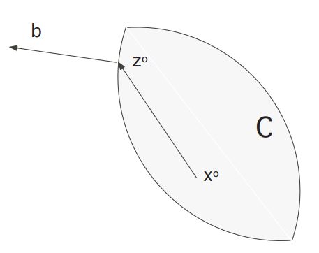
1. If $\mathcal{C}\ne {\mathbb{R}}^n$, then the convexity of $\mathcal{C}$ implies that there exists a vector $b\ne 0$ and a real number $\mu$ s.t.

$$b\cdot x^0\le \mu ,\mathrm{\forall }{x}^0\in \mathcal{C}$$

(Must contain a support hyperplane if $\mathcal{C}$ doesn't contain the whole space)

Indeed, in the picture we see that $b\cdot (x^0-z^0)\le 0$; and this implies that $\mu :=b\cdot z^0$.

We will derive a contradiction.

2. Given $b\ne 0,\mu \in \mathbb{R}$, our intention is to find $x^0\in \mathcal{C}$ s.t. $b\cdot x^0\le \mu$ fails. Recall $x^0\in \mathcal{C}$ iff $\mathrm{\exists }t>0$ and a control $\mathit{\alpha }(\cdot )\in \mathcal{A}$ s.t.

$$x^0=-{\int }_0^t{\mathit{X}}^{-1}(s)N\mathit{\alpha }(s)\mathrm{d}s$$

Then

$$b\cdot x^0=-{\int }_0^t{b}^{\mathrm{\top }}{\mathit{X}}^{-1}(s)N\mathit{\alpha }(s)\mathrm{d}s$$

Define

$$\mathit{v}(s):=b^{\mathrm{\top }}{\mathit{X}}^{-1}(s)N$$

3. We assert that $\mathit{v}\ne 0$

To see this, suppose instead that $\mathit{v}\equiv 0$. Then $k$ times differentiate the expression $b^{\mathrm{\top }}{\mathit{X}}^{-1}(s)N$ w.r.t. $s$ and set $s=0$, to discover

$$b^{\mathrm{\top }}{M}^{k}N=0,k=0,1,2,\dots$$

This implies $b$ is orthogonal to the columns of $G$, and so $\mathrm{rank}G<n$. This is a contradiction to our hypothesis, and therefore $\mathit{v}\ne 0$ holds.

4. Next, define $\mathit{\alpha }(\cdot )$ this ay:

$$\mathit{\alpha }(s):=\{\begin{array}{ll}-\frac{\mathit{v}(s)}{|\mathit{v}(s)|},& \text{if }\mathit{v}(s)\ne 0,\\ 0,& \text{if }\mathit{v}(s)=0.\end{array}$$

Then

$$b\cdot x^0=-{\int }_0^t\mathit{v}(s)\mathit{\alpha }(s)\mathrm{d}s={\int }_0^t|\mathit{v}(s)|\mathrm{d}s$$

We want to find a time $t>0$ s.t. ${\int }_0^t|\mathit{v}(s)|\mathrm{d}s>\mu$. In fact, we assert that

$${\int }_0^{\mathrm{\infty }}|\mathit{v}(s)|\mathrm{d}s=+\mathrm{\infty }$$

To begin the proof above introduce the function

$$\varphi (t):={\int }_t^{\mathrm{\infty }}\mathit{v}(s)\mathrm{d}s$$

We will find an ODE $\varphi$ satisfies. Take $p(\cdot )$ to be the characteristic polynomial of $M$. Then

$$\begin{array}{rl}& p(-\frac{\mathrm{d}}{\mathrm{d}t})\mathit{v}(t)\\ =& p(-\frac{\mathrm{d}}{\mathrm{d}t})[b^{\mathrm{\top }}{e}^{-tM}N]\\ =& b^{\mathrm{\top }}\left(p(-\frac{\mathrm{d}}{\mathrm{d}t})e^{-tM}\right)N\\ =& b^{\mathrm{\top }}\left(p\left(M\right)e^{-tM}\right)N\equiv 0\end{array}$$

Since $p(M)=0$, according to the Cayley–Hamilton Theorem. But since $p(-\frac{\mathrm{d}}{\mathrm{d}t})\mathit{v}(t)\equiv 0$, it follows that

$$-\frac{\mathrm{d}}{\mathrm{d}t}p(-\frac{\mathrm{d}}{\mathrm{d}t})\varphi (t)=p(-\frac{\mathrm{d}}{\mathrm{d}t})(-\frac{\mathrm{d}}{\mathrm{d}t}\varphi )=p(-\frac{\mathrm{d}}{\mathrm{d}t})\mathit{v}(t)=0$$

Hence $\varphi$ solves the (n+1)th order ODE

$$\frac{\mathrm{d}}{\mathrm{d}t}p(-\frac{\mathrm{d}}{\mathrm{d}t})\varphi (t)=0$$

We also know that $\varphi (\cdot )\ne 0$. Let ${\mu }_1,\cdots ,{\mu }_{n+1}$ be the solutions of $\mu p(-\mu )=0$. According to ODE theory, we can write

$$\varphi (t)=\text{sum of the terms of the form }{p}_i(t)e^{{\mu }_{i}t}$$

for appropriate polynomials $p_i(\cdot )$

Furthermore, we see that ${\mu }_{n+1}=0$ and ${\mu }_k=-{\lambda }_k$, where ${\lambda }_1,\cdots ,{\lambda }_n$ are the eigenvalues of $M$. By assumption $\mathrm{Re}{\mu }_k\ge 0,k=0,1,\cdots ,n$. If ${\int }_0^{\mathrm{\infty }}|\mathit{v}(s)|\mathrm{d}s<\mathrm{\infty }$, then

$$|\varphi (t)|\le {\int }_0^{\mathrm{\infty }}|\mathit{v}(s)|\mathrm{d}s\to 0,\text{as }t\to \mathrm{\infty }$$

that is, $\varphi (t)\to 0$ as $t\to \mathrm{\infty }$. This's a contradiction to the representation formula of $\varphi (t)=\sum p_i(t)e^{{\mu }_{i}t}$, with $\mathrm{Re}{\mu }_i\ge 0$. Assertaion is proved.

5. Consequently given any $\mu ,\mathrm{\exists }t>0$ s.t.

$$b\cdot x^0={\int }_0^t|\mathit{v}(s)|\mathrm{d}s>\mu$$

a contradiction to (2.8). Therefore $\mathcal{C}={\mathbb{R}}^n$.

$◻$

2.4 Observability

Consider the linear system of ODE

$$\{\begin{array}{l}\dot{\mathit{x}}(t)=M\mathit{x}(t)\\ \mathit{x}(0)=x^0.\end{array}$$

where $M\in {\mathbb{M}}^{n\times n}$.

In this section we address the observability problem, modeled as follows. We suppose that we can observe

$$\mathit{y}(t):=N\mathit{x}(t)(t\ge 0)$$

for a given matrix $N\in {\mathbb{M}}^{m\times n}$. Consequently, $\mathit{y}(t)\in {\mathbb{R}}^m$. The interesting situation is when $m<<n$ and we interpret $\mathit{y}(\cdot )$ as low-dimensional “observations” or “measurements” of the high-dimensional dynamics $\mathit{x}(\cdot )$

Observability question: Given the observation $\mathit{y}(\cdot )$, can we in principle reconstruct $\mathit{x}(\cdot )$? In particular, do observations of $\mathit{y}(\cdot )$ provide enough information for us to deduce the initial value $x^0$ for (ODE)?

Definition: observable

The pair (ODE, Observation) called observable if the knowledge of $\mathit{y}(\cdot )$ on any time interval $[0,t]$ allows us to compute $x^0$.

More precisely, (ODE, Observation) is observable if for all solutions ${\mathit{x}}_1(\cdot ),{\mathit{x}}_2(\cdot ),N{\mathit{x}}_1(\cdot )\equiv N{\mathit{x}}_2(\cdot )$ on a time interval $[0,t]$ implies ${\mathit{x}}_1(0)={\mathit{x}}_2(0)$.

2 simple examples

1. If $N\equiv 0$, then clearly the system is not observable.
2. On the other hand, if $m=n$ and $N$ is invertible, then clearly $\mathit{x}(t)=N^{-1}\mathit{y}(t)$ is observable.

The interesting cases lie between these extremes.

Theorem 2.7: Observability and controllability The system 1

$$\{\begin{array}{l}\dot{\mathit{x}}(t)=M\mathit{x}(t)\\ \mathit{y}(t)=N\mathit{x}(t)\end{array}$$

is observable iff the system 2

$$\dot{\mathit{z}}(t)=M^{\mathrm{\top }}\mathit{z}(t)+N^{\mathrm{\top }}\mathit{\alpha }(t),A={\mathbb{R}}^m$$

is controllable, meaning that $\mathcal{C}={\mathbb{R}}^n$

INTERPRETATION. This theorem asserts that somehow “observability and controllability are dual concepts” for linear systems.

Proof:

1. ($\leftarrow$) Suppose the system 1 is not observable. Then $\mathrm{\exists }{x}^1\ne x^2\in {\mathbb{R}}^n$, s.t.

   $$\{\begin{array}{l}{\dot{\mathit{x}}}_1(t)=M{\mathit{x}}_1(t),{\mathit{x}}_1(0)=x^1\\ {\dot{\mathit{x}}}_2(t)=M{\mathit{x}}_2(t),{\mathit{x}}_2(0)=x^2\end{array}$$

but $\mathit{y}(t):=N{\mathit{x}}_1(t)\equiv N{\mathit{x}}_2(t),\mathrm{\forall }t\ge 0$. Let

$$\mathit{x}(t):={\mathit{x}}_1(t)-{\mathit{x}}_2(t),x^0:=x^1-x^2$$

Then

$$\dot{\mathit{x}}(t)=M\mathit{x}(t),\mathit{x}(0)=x^0\ne 0$$

but

$$N\mathit{x}(t)=0(t\ge 0)$$

Now

$$\mathit{x}(t)=\mathit{X}(t)x^0=e^{tM}{x}^0$$

Thus

$$N{e}^{tM}{x}^0=0(t\ge 0)$$

Let $t=0$, to find $N{x}^0=0$. Then differentiate this expression $k$ times in $t$ and let $t=0$, to discover as well that

$$N{M}^k{x}^0=0$$

for $k=0,1,2\cdots$ Hence $(x^0{)}^{\mathrm{\top }}(M^k{)}^{\mathrm{\top }}{N}^{\mathrm{\top }}=0$ and hence $(x^0{)}^{\mathrm{\top }}(M^{\mathrm{\top }}{)}^k{N}^{\mathrm{\top }}=0$. This implies

$$(x^0{)}^{\mathrm{\top }}[N^{\mathrm{\top }},M^{\mathrm{\top }}{N}^{\mathrm{\top }},\cdots ,(M^{\mathrm{\top }}{)}^{n-1}{N}^{\mathrm{\top }}]=0$$

Since $x^0\ne 0,\mathrm{rank}[N^{\mathrm{\top }},\cdots ,(M^{\mathrm{\top }}{)}^{n-1}{N}^{\mathrm{\top }}]<n$. Thus system 2 is not controllable. Consequently, system 2 controllable implies system 1 is observable.

2. ($\to$)Assume now system 2 is not controllable. Then $\mathrm{rank}[N^{\mathrm{\top }},\cdots ,(M^{\mathrm{\top }}{)}^{n-1}{N}^{\mathrm{\top }}]<n$, and consequently according to Theorem 2.3, $\mathrm{\exists }{x}^0\ne 0$, s.t.

$$(x^0{)}^{\mathrm{\top }}[N^{\mathrm{\top }},\cdots ,(M^{\mathrm{\top }}{)}^{n-1}{N}^{\mathrm{\top }}]=0$$

That is, $N{M}^k{x}^0=0,\mathrm{\forall }k=0,1,2,\cdots ,n-1$

We want to show that $\mathit{y}(t)=N\mathit{x}(t)\equiv 0$, where

$$\{\begin{array}{l}\dot{\mathit{x}}(t)=M\mathit{x}(t)\\ \mathit{x}(0)=x^0.\end{array}$$

According to the Cayley–Hamilton Theorem, we can write

$$M^n=-{\beta }_{n-1}{M}^{n-1}-\cdots -{\beta }_{0}I$$

for appropriate constants. Consequently $N{M}^n{x}^0=0$. Likewise

$$\begin{array}{rl}{M}^{n+1}& =M(-{\beta }_{n-1}{M}^{n-1}-\cdots -{\beta }_{0}I)\\ & =-{\beta }_{n-1}{M}^n-\cdots -{\beta }_{0}M\end{array}$$

and so $N{M}^{n+1}{x}^0=0$. Similarly, $N{M}^k{x}^0=0,\mathrm{\forall }k$.

Now

$$\mathit{x}(t)=\mathit{X}(t)x^0=e^{Mt}{x}^0=\sum _{k=0}^{\mathrm{\infty }}\frac{t^k{M}^k}{k!}{x}^0$$

and therefore $N\mathit{x}(t)=N\sum _{k=0}^{\mathrm{\infty }}\frac{t^k{M}^k}{k!}{x}^0=0$

We have shown that if system 2 is not controllable, then system 1 is not observable.

$◻$

2.5 bang-bang control

Again take $A$ to be the cube $[-1,1{]}^m\in {\mathbb{R}}^m$.

Definition: bang-bang

A control $\mathit{\alpha }(\cdot )\in \mathcal{A}$ is called bang-bang if $\mathrm{\forall }t\ge 0$ and for each index $i=1,\cdots ,m$, we have $|{\alpha }^i(t)|=1$, where

$$\mathit{\alpha }(t)={\left[\begin{array}{ccc}{\alpha }^1(t)& \cdots & {\alpha }^m(t)\end{array}\right]}^{\mathrm{\top }}$$

Theorem 2.8: bang-bang principle

Let $t>0$ and suppose $x^0\in \mathcal{C}(t)$, for the system

$$\dot{\mathit{x}}(t)=M\mathit{x}(t)+N\mathit{\alpha }(t).$$

Then there exists a bang-bang control $\mathit{\alpha }(\cdot )$ which steers $x^0$ to $0$ at time $t$.

To prove the theorem we need some tools from functional analysis, among them the Krein–Milman Theorem, expressing the geometric fact that every bounded convex set has an extreme point.

2.5.1 Some functional analysis

We will study the “geometry” of certain infinite dimensional spaces of functions.

Notation

$$\begin{array}{c}{L}^{\mathrm{\infty }}=L^{\mathrm{\infty }}(0,t;{\mathbb{R}}^m)=\{\mathit{\alpha }(\cdot ):(0,t)\to {\mathbb{R}}^m|\underset{0\le s\le t}{sup}|\mathit{\alpha }(s)|<\mathrm{\infty }\}.\\ \parallel \mathit{\alpha }{\parallel }_{L^{\mathrm{\infty }}}=\underset{0\le s\le t}{sup}|\mathit{\alpha }(s)|.\end{array}$$

Definition: converge in the weak* sense

Let $\mathit{\alpha }\in L^{\mathrm{\infty }}$ for $n=1,\cdots$ and $\mathit{\alpha }\in L^{\mathrm{\infty }}$. We say ${\mathit{\alpha }}_n$ converges to $\mathit{\alpha }$ in the weak* sense, written

$${\mathit{\alpha }}_n\stackrel{\ast }{\rightharpoonup }\mathit{\alpha }.$$

provided

$${\int }_0^t{\mathit{\alpha }}_n(s)\cdot \mathbf{v}(s)\mathrm{d}s\to {\int }_0^t\mathit{\alpha }(s)\cdot \mathbf{v}(s)\mathrm{d}s$$

as $n\to \mathrm{\infty }$, for all $\mathit{v}(\cdot ):[0,t]\to {\mathbb{R}}^m$ satisfying ${\int }_0^t|\mathbf{v}(s)|\mathrm{d}s<\mathrm{\infty }$.

We will the following useful weak* compactness theorem for $L^{\mathrm{\infty }}$.

Alaoglu's Theorem

Let ${\mathit{\alpha }}_n\in \mathcal{A},n=1,\cdots$. Then there exists a subsequence ${\mathit{\alpha }}_{n_k}$ and $\mathit{\alpha }\in \mathcal{A}$ s.t.

$${\mathit{\alpha }}_{n_k}\stackrel{\ast }{\rightharpoonup }\mathit{\alpha }.$$

Definition: convex; extreme point

• The set $\mathbb{K}$ is convex if $\mathrm{\forall }x,\hat{x}\in \mathbb{K}$ and all real numbers $0\le \lambda \le 1$,

  $$\lambda x+(1-\lambda )\hat{x}\in \mathbb{K}.$$

• A point $z\in \mathbb{K}$ called extreme provided there do not exist points $x,\hat{x}\in \mathbb{K}$ and $0<\lambda <1$ s.t.

  $$z=\lambda x+(1-\lambda )\hat{x}.$$

Krein-Milman Theorem

Let $\mathbb{K}$ be a convex, nonempty subset of $L^{\mathrm{\infty }}$, which is compact in the weak* topology.

Then $\mathbb{K}$ has at least one extreme point.

2.5.2 Application to bang-bang control

The foregoing abstract theory will be useful for us in the following setting. We will take $\mathbb{K}$ to be the set of controls which steer $x^0$ to $0$ at time $t$, prove it satisfies the hypotheses of Krein–Milman Theorem and finally show that an extreme point is a bang-bang control.

So consider again the linear dynamics

$$\{\begin{array}{l}\dot{\mathit{x}}(t)=M\mathit{x}(t)+N\mathit{\alpha }(t)\\ \mathit{x}(0)=x^0.\end{array}$$

take $x^0\in \mathcal{C}(t)$ and write

$$\mathbb{K}=\{\mathit{\alpha }(\cdot )\in \mathcal{A}|\mathit{\alpha }(\cdot )\text{ steers }{x}^0\text{ to }0\text{ in time }t\}.$$

Lemma 2.9: Geometry of set of controls

The collection $\mathbb{K}$ of admissible controls satisfies the hypotheses of the Krein-Milman Theorem.

Proof: Since $x^0\in \mathcal{C}(t)$, we see that $\mathbb{K}\notin \varphi$.

Next we show that $\mathbb{K}$ is convex. For this, recall that $\mathit{\alpha }(\cdot )\in \mathbb{K}$ iff

$$x^0=-{\int }_0^t{\mathit{X}}^{-1}(s)N\mathit{\alpha }(s)\mathrm{d}s.$$

Now take also $\hat{\mathit{\alpha }}\in \mathbb{K}$ and $0\le \lambda \le 1$. Then

$$x^0=-{\int }_0^t{\mathit{X}}^{-1}(s)N\hat{\mathit{\alpha }}(s)\mathrm{d}s.$$

and so

$$x^0=-{\int }_0^t{\mathit{X}}^{-1}(s)N(\mathit{\alpha }(s)+(1-\lambda )\hat{\mathit{\alpha }}(s))\mathrm{d}s.$$

Hence $\lambda \mathit{\alpha }+(1-\lambda )\hat{\mathit{\alpha }}\in \mathbb{K}$.

Lastly, we confirm the compactness. Let ${\mathit{\alpha }}_n\in \mathbb{K}$ for $n=1,\cdots$. According to Alaoglu’s Theorem $\mathrm{\exists }{n}_k\to \mathrm{\infty }$ and $\mathit{\alpha }\in \mathcal{A}$ s.t. ${\mathit{\alpha }}_{n_k}\stackrel{\ast }{\rightharpoonup }\mathit{\alpha }$. We need to show that $\mathit{\alpha }\in \mathbb{K}$.

Now ${\mathit{\alpha }}_{n_k}\in \mathbb{K}$ implies

$$x^0=-{\int }_0^t{\mathit{X}}^{-1}(s)N{\mathit{\alpha }}_{n_k}(s)\mathrm{d}s\to -{\int }_0^t{\mathit{X}}^{-1}(s)N\mathit{\alpha }(s)\mathrm{d}s.$$

by definition of weak-* convergence. Hence $\mathit{\alpha }\in \mathbb{K}.$

$◻$

We can now apply the Krein–Milman Theorem to deduce that there exists an extreme point $\mathit{\alpha }\in \mathbb{K}$. What is interesting is that such an extreme point corresponds to a bang-bang control.

Theorem 2.10: Extremality and bang-bang principle

The control $\mathit{\alpha }(\cdot )$ is bang-bang.

Proof:

1. We must show that for almost all times $0\le s\le t$ and for each $i=1,\cdots ,m$, we have

$$|{\alpha }^{i\ast }(s)|=1.$$

Suppose not. Then there exists an index $i\in \{1,\cdots ,m\}$ and a subset $E\subset [0,t]$ of positive measure s.t. $|{\alpha }^{i\ast }(s)|<1$ for $s\in E$. In fact, $\mathrm{\exists }\epsilon >0$ and a subset $F\subseteq E$ s.t.

$$|F|>0\text{ and }|{\alpha }^{i\ast }(s)|\le 1-\epsilon \text{ for }s\in F.$$

Define

$$I_F(\beta (\cdot )):={\int }_F{\mathit{X}}^{-1}(s)N\mathit{\beta }(s)\mathrm{d}s.$$

for $\mathit{\beta }=(0,\cdots ,\beta (\cdot ),\cdots ,0{)}^{\mathrm{\top }}.$, the function $\beta$ in the $i^{\mathrm{th}}$ slot. Choose any real-valued function $\beta (\cdot )\not\equiv 0$, s.t.

$$I_F(\beta (\cdot ))=0$$

and $|\beta (\cdot )|\le 1$. Define

$$\begin{array}{rl}{\mathit{\alpha }}_1(\cdot )& :={\mathit{\alpha }}^{\ast }(\cdot )+\epsilon \mathit{\beta }(\cdot )\\ {\mathit{\alpha }}_2(\cdot )& :={\mathit{\alpha }}^{\ast }(\cdot )-\epsilon \mathit{\beta }(\cdot ),\end{array}$$

where we redefine $\beta$ to be zero off the set $F$

2. We claim that ${\mathit{\alpha }}_1(\cdot ),{\mathit{\alpha }}_2(\cdot )\in \mathbb{K}$.

To see this, observe that

$$\begin{array}{rl}& -{\int }_0^t{\mathbf{X}}^{-1}(s)N{\mathit{\alpha }}_1(s)\mathrm{d}s\\ =& -{\int }_0^t{\mathbf{X}}^{-1}(s)N{\mathit{\alpha }}^{\ast }(s)\mathrm{d}s-\epsilon {\int }_0^t{\mathbf{X}}^{-1}(s)N\mathit{\beta }(s)\mathrm{d}s\\ =& x^0-\epsilon \underset{I_F(\beta (\cdot ))=0}{\underbrace{{\int }_F{\mathbf{X}}^{-1}(s)N\mathit{\beta }(s)\mathrm{d}s}}=x^0\end{array}$$

Note also ${\mathit{\alpha }}_1(\cdot )\in \mathcal{A}$. Indeed,

$$\{\begin{array}{ll}{\mathit{\alpha }}_1(s)={\mathit{\alpha }}^{\ast }(s)& (s\notin F)\\ {\mathit{\alpha }}_1(s)={\mathit{\alpha }}^{\ast }(s)+\epsilon \mathit{\beta }(s)& (s\in F).\end{array}$$

But on the set $F$, we have $|{\mathit{\alpha }}_i^{\ast }(s)|\le 1-\epsilon$, and therefore

$$|{\mathit{\alpha }}_1(s)|\le |{\mathit{\alpha }}^{\ast }(s)|+\epsilon |\mathit{\beta }(s)|\le 1-\epsilon +\epsilon =1\text{. }$$

Similar considerations apply for ${\mathit{\alpha }}_2$. Hence ${\mathit{\alpha }}_1,{\mathit{\alpha }}_2\in \mathbb{K}$, as claimed above.

3. Finally, observe that

$$\begin{array}{rlr}{\mathit{\alpha }}_1(\cdot )& ={\mathit{\alpha }}^{\ast }+\epsilon \mathit{\beta },& {\mathit{\alpha }}_1\ne {\mathit{\alpha }}^{\ast }\\ {\mathit{\alpha }}_2(\cdot )& ={\mathit{\alpha }}^{\ast }-\epsilon \mathit{\beta },& {\mathit{\alpha }}_2\ne {\mathit{\alpha }}^{\ast }\end{array}$$

But

$$\frac{1}{2}{\mathit{\alpha }}_1+\frac{1}{2}{\mathit{\alpha }}_2={\mathit{\alpha }}^{\ast }.$$

and this is a contradiction, since ${\mathit{\alpha }}^{\ast }$ is an extreme point of $\mathbb{K}$.

$◻$