Skip to content

Laplace Transform ​

Formulation & Definition ​

Introduction ​

In mathematics, the Laplace transform, named after its inventor Pierre-Simon Laplace is an integral transform that converts a function of a real variable t (often time) to a function of a complex variable s (complex frequency).

For suitable functions f, the Laplace transform is the integral

L{f}(s)=∫0∞f(t)e−st dt.

Here's the Fourier Transformation (for real number):

F(ω)=F(f(t))=∫0∞f(t)e−iωt dt.

Why do we need Laplace Transform for solving ODE? ​
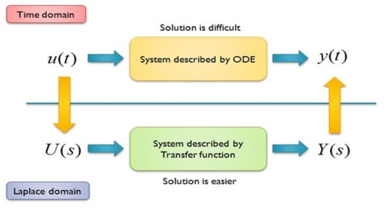
Why using laplace transform

The Formulation of Laplace Transform ​

Definition: Laplace Transform

If a function f(t) is multiplied by e−st, and the result is integrated with respect to t from t=0 to t=∞, a new function of the variable s is obtained when the integral exists.

This function (when it exists) is called the Laplace transform of f(t):

L{f}(s)=∫0∞f(t)e−st dt.

Suppose that we require the solution of the differential equation:

dydt−y=eat

for positive values of t, which satisfies the initial condition

y(0)=−1.
dydt−y=eat⟹Letp=exp⁡(∫−1 dt)=exp⁡(−t)⟹y=1p∫peat dt+cexp⁡(−t)y=exp⁡(t)∫exp⁡(−t+at) dt+cexp⁡(t)y=exp⁡(t)(c+1a−1exp⁡((a−1)t))y(0)=−1⟹c=−1−1a−1=−aa−1⟹y=exp⁡(t)(−aa−1+1a−1exp⁡((a−1)t))y=1a−1(exp⁡(at)−aexp⁡(t))
  1. We first take the Laplace transform of both sides of the previous equation, by multiplying both sides of the equation by e−st and integrating the results with respect to t from zero to infinity,
∫0∞e−stdydt dt−∫0∞e−sty dt=∫0∞e−steat dt
  1. The integral on the right is readily evaluated
∫0∞e−steat dt=−e−(s−a)ts−a|0∞=1s−a

the integral exists when s>a. The first integral on the left can be integrated formally by parts to give

∫0∞e−stdydt dt=e−sty(t)|0∞+s∫0∞e−sty dt=−y(0)+s∫0∞e−sty dt=1+s∫0∞e−sty dt
  1. As a result, we obtain
(s−1)∫0∞e−sty dt=1s−a−1 or ∫0∞e−sty dt=a+1−s(s−1)(s−a)
  1. Expand this expression by the method of partial fractions, to obtain the equivalent form
∫0∞e−sty dt=1a−11s−a−aa−11s−1
  1. Reference to ∫0∞e−teat dt=−e−(−b−a)ts−a|0∞=1s−a, then indicates that, since 1/(s−a) is the transform of eat, the first term is the transform of eat/(a−1) and the second term the transform of −aet/(a−1).

  2. The original problem is now apparently reduced to the problem of determining a function y(t) whose Laplace transform is given by the above equation

  3. Applying the inverse Laplace transform, one can obtain for a≠1

y=1a−1(eat−aet)

or for a=1, can be obtained by taking the limit as a→1

y=(t−1)et

Definition of Laplace Transform ​

The Laplace transform of a function f(t), defined for positive values of t, is frequently indicated by the notation L{f(t)} and is defined, as a function of the variable s, by the integral

L{f(t)}=∫0∞f(t)e−st dt.

over that range of values of s for which the integral exists.

The notation f¯(s) or merely f¯ is also used in place of L{f(t)}.

The Existence of Laplace Transform ​

  • Integration may fail to define a function of s, in particular, because of infinite discontinuities in f(t) for certain positive values of t or because of failure of f(t) to behave in a sufficiently regular way near t=0 or for large values of t. However, the presence of a finite number of finite discontinuities or "jumps" will not, in itself, affect the existence of the integral
  • A function f(t) is said to be piecewise continuous in a finite range if it is possible to divide that range into a finite number of intervals such that f(t) is continuous inside each interval and approaches finite values as either end of any interval is approached from the interior. Such functions may thus have finite jumps at points inside the range considered
L{f(t)}=∫0∞f(t)e−st dt=(∫0t1+∫t1T+∫T∞)f(t)e−st dt

Sufficient additional condition to guarantee the existence of the third integral item L{f(t)}=∫T∞f(t)e−st dt, at least for sufficiently large values of s, is the requirement that f(t) belong to the rather extensive class of "functions of exponential order".

A function f(t) is said to be of exponential order if, for some number s0, the product e−s0t|f(t)| is bounded for large values of t, say for t>T.

If the bound is denoted by M, then there follows, when t>T:

e−s0t|f(t)|<M, or |f(t)|<Mes0t.⟹|e−stf(t)|<e−st⋅Mes0t=Me−(s−s0)t

the Laplace transform of f(t) exists, when s is sufficiently large, if f(t) satisfies the following conditions:

  • f(t) is continuous or piecewise continuous in every finite interval t1⩽t⩽T, where t1>0.
  • tn|f(t)| is bounded near t=0 for some number n, where n<1.
  • e−s0t|f(t)| is bounded for large values of t, for some number s0.

Examples for Laplace Transforms ​

L{1}=∫0∞e−st dt=−e−sts|0∞=1s(s>0).L{eat}=∫0∞e−(s−a)t dt=−e−(s−a)ts−a|0∞=1s−a(s>a).L{sin⁡at}=∫0∞e−stsin⁡at dt=−e−sts2+a2(ssin⁡at+acos⁡at)|0∞=as2+a2(s>0).

Properties [core] ​

Properties of Laplace Transform ​

Some most useful properties of Laplace transforms:

  1. Linearity
L{af(t)+bg(t)}=af¯(s)+bg¯(s)
  1. n-order derivative of function
L{dnf(t)dtn}=snf¯(s)−[sn−1f(0+)+sn−2df(0+)dt+sn−3d2f(0+)dt2+⋯+dn−1f(0+)dtn−1]
L{df(t)dt}=∫0∞e−stdf(t)dt dt

An integration by parts gives

∫0∞e−stdf(t)dt dt=e−stf(t)|0∞+s∫0∞e−stf(t) dt

if f(t) is continuous and df(t)dt is piecewise continuous in every interval But since f(t) is of exponential order, the integrated part vanishes as (for s>s0 ), and there follows

L{df(t)dt}=sf¯(s)−f(0+)L{d2f(t)dt2}=∫0∞e−std2f(t)dt2 dt=e−stdf(t)dt|0∞+s∫0∞e−stdf(t)dt dt=e−stdf(t)dt|0∞+sL{df(t)dt}L{d2f(t)dt2}=s2f¯(s)−sf(0+)−df(0+)dt
  1. Integration of function
L{∫0tf(u) du}=1sf¯(s)
L{∫0tf(u) du}=∫0∞e−st{∫0tf(u) du} dt=[e−st−s∫0tf(u) du]0∞+1s∫0∞e−stf(t) dt=1sf¯(s)

the integrated part vanishing at the upper limit (for sufficiently large values of s ), since f(t), and hence ∫0tf(u) du, is of exponential order. Thus, in general, if a function is integrated over (0,t), the transform of the integral is obtained by dividing the transform of the function by s.

If the lower limit differs from zero, the formula

L{∫atf(u) du}=1sf¯(s)−1s∫0af(u) du

is easily established.

  1. Shifting of function (after LT)
L{eatf(t)}=f¯(s−a)

If f(t)={0,t<ag(t−a),t≧a} with a≧0, then f¯(s)=e−asg¯(s).

  1. Derivative of function after LT
L{tnf(t)}=(−1)ndnf¯(s)dsn
  1. Convolution of function: Multiplication of two functions after LT
L{∫0tf(t−u)g(u) du}=f¯(s)g¯(s)

In these equations a and b are constants, and n is a positive integer.

The Convolution Properity ​

L{∫0tf(t−u)g(u) du}=f¯(s)g¯(s)f¯(s)g¯(s)=[∫0∞e−svf(v) dv][∫0∞e−sug(u) du]=∫0∞∫0∞e−s(v+u)f(v)g(u) dv du=∫0∞g(u){∫0∞e−s(v+u)f(v) dv} du

if different "dummy variables" of integration ( v and u ) are used in defining the two transforms. If, in the inner integral of the last form, we replace v by a new variable t with the substitution

v=t−u,dv=dt,

there follows

∫0∞e−s(v+u)f(v) dv=∫u∞e−stf(t−u) dt

and hence

f¯(s)g¯(s)=∫0∞g(u){∫u∞e−stf(t−u) dt} du=∫0∞e−st{∫0tf(t−u)g(u) du} dt=L{∫0tf(t−u)g(u) du}.conv

Inversion of Laplace Transform ​

Inverse of the Laplace Transform ​

To determine the inverse transform of a given function F(s) it is thus necessary to determine a function f(t) which satisfies the equation

∫0∞e−stf(t) dt=F(s).⟺f(t)=L−1{F(s)}.

Since the unknown function f(t) appears under an integral sign, an equation of this type is called an integral equation.

In more advanced works it is proved that if this equation has a solution, then that solution is unique. Thus, if one function having a given transform is known, it is the only possible one. This result is known as Lerch's theorem.

More precisely, Lerch's theorem states that two functions having the same transform cannot differ throughout any interval of positive length. Thus, for example, it's shown that the continuous solution of

∫0∞e−stf(t) dt=1s

is f(t)=1; that is, L−1{s−1}=1. However, it is clear that if we take f(t) to be, say, zero at t=1 and unity elsewhere, or otherwise redefine the function f(t) at a finite number of points, the value of the integral is not changed. Hence the new function is also a solution. Such artificialities are, however, generally of no significance in applications.

Table: Laplace Transform [core]

TransformFunction
T1f¯(s)=L{f(t)}=∫0∞e−stf(t) dtf(t)
T2af¯(s)+bg¯(s)af(t)+bg(t)
T3sf¯(s)−f(0)df(t)dt
T4s2f¯(s)−sf(0)−df(0)dtd2f(t)dt2
T5snf¯(s)−∑k=1nsn−kdk−1f(0)dtk−1dnf(t)dtn
T61snf¯(s)∫0t⋯∫0t⏞n times f(t)dt⋯dt⏞n times 
T7(−1)ndnf¯(s)dsntnf(t)
T8f¯(s−a)eatf(t)
T9e−asf¯(s){f(t−a)(t>a)0(t<a)
T10f¯(s)g¯(s)∫0tf(t−u)g(u)du=∫0tf(u)g(t−u)du
T111s1
T121s+ae−at
T131(s+a)(s+b)1a−b(e−bt−e−at)
T14s(s+a)(s+b)1b−a(be−bt−ae−at)
T15as2+a2sin⁡at
T16ss2+a2cos⁡at
T17as2−a2sinh⁡at
T18ss2−a2cosh⁡at
T192as(s2+a2)2tsin⁡at
T20s2−a2(s2+a2)2tcos⁡at
T212a3(s2+a2)2sin⁡at−atcos⁡at
T222as(s2−a2)2tsinh⁡at
T23s2+a2(s2−a2)2tcosh⁡at
T242a3(s2−a2)2atcosh⁡at−sinh⁡at
T25a(s+b)2+a2e−btsin⁡at
T26s+b(s+b)2+a2e−btcos⁡at
T274c3s4+4a4sin⁡atcosh⁡at−cos⁡atsinh⁡at
T282a2ss4+4a1sin⁡atsinh⁡at
T292a3s4−a4sinh⁡at−sin⁡at
T302a1ss4−a4cosh⁡at−cos⁡at
T311δ(t)
T32e−st1δ(t−t1)
T33sδ′(t)
T34se−st1δ′(t−t1)
T351sntn−1(n−1)!
T35an!sn+1tn
T361(s+a)ntn−1e−at(n−1)!
T37s(s+a)n(n−1)−at(n−1)!tn−2e−at
T38a2n−1(s2+a2)n12n−1(n−1)![π2(at)n−1/2Jn−1/2(at)](n>0)
T39a2n−2s(s2+a2)nat2n(n−1)![π2(at)n−3/2Jn−3/2(at)](n>12)
T40a2n−1(s2−a2)n12n−1(n−1)![π2(at)n−1/2In−1/2(at)](n>0)
T41a2n−2s(s2−a2)nat2n(n−1)![π2(at)n−3/2In−3/2(at)](n>12)

Table: Bessel functions of order half an odd integer

mπ2xmJm(x)π2xmIm(x)
-1/2(cos⁡x)/x(cosh⁡x)/x
12sin⁡xsinh⁡x
32sin⁡x−xcos⁡xxcosh⁡x−sinh⁡x
52(3−xx)sin⁡x−3xcos⁡x(3+x2)sinh⁡x−3xcosh⁡x
7/2(15−6x2)sin⁡x−(15−x2)xcos⁡x(15+x2)xcosh⁡x−(15+6x2)sinh⁡x
92(105−45x2+1)sin⁡x−(105−10x2)xcos⁡x(105+45x2+1)sinh⁡x−(105+10x2)xcosh⁡x
Recurrence Formulas
xm+1Jm+1(x)=2m[xmJm(x)]−x2[xm−1Jm−1(x)]xm+1Im+1(x)=−2m[xmIm(x)]+x2[xm−1Im−1(x)]

Method of Partial Fractions for the Inverse of Laplace Transform ​

For

F(s)=N(s)D(s)

where D(s) is a polynomial of degree n with n distinct real zeros s=a1,a2,⋯an, and N(s) is a polynomial of degree n−1 or less, there follows

N(s)D(s)=N(a1)D′(a1)1s−a1+N(a2)D′(a2)1s−a2+⋯+N(an)D′(an)1s−an=∑m=1nN(am)D′(am)1s−am

(Heaviside cover-up method / Residue Method) Let

N(s)D(s)=∑m=1nAms−am⟹(s−ak)N(s)D(s)=Ak+∑m=1,m≠knAms−aks−am⟹lims→ak(s−ak)N(s)D(s)=lims→ak(Ak+∑m=1,m≠knAms−aks−am)lims→akN(s)D(s)−D(ak)s−ak=Ak⟹N(ak)D′(ak)=Ak.

With M-fold roots, like only ak, i.e. (s−ak)M:

N(s)D(s)=∑m=1,m≠knN(am)D′(am)1s−am+∑m=1M1(M−m)!d(n−k)dx(n−k)(N(s)D(s)(x−ak)n)1(s−ak)m.

and hence, from (T12),

L−1{N(s)D(s)}=∑m=1nN(am)D′(am)eamt

Example1: Inverse Laplace Transform ​

To determine L−1{s2+1s3+3s2+2s}, we write

N(s)=s2+1,D(s)=s3+3s2+2s=s(s+1)(s+2)

With a1=0,a2=−1,a3=−2, and D′=3s2+6s+2, there follows

N(a1)=1,D′(a1)=2,N(a2)=2,D′(a2)=−1,N(a3)=5,D′(a3)=2,L−1{s2+1s3+3s2+2s}=12−2e−t+52e−2t.

Example2: Inverse Laplace Transform ​

To determine L−1{ss2+4s+5}, we first write

ss2+4s+5=s(s+2)2+1=(s+2)−2(s+2)2+1.

Pairs (T25,26) then give the required inverse transform

e−2t(cos⁡t−2sin⁡t).

Example3: Solving the following ODE with Laplace Transform [core] ​
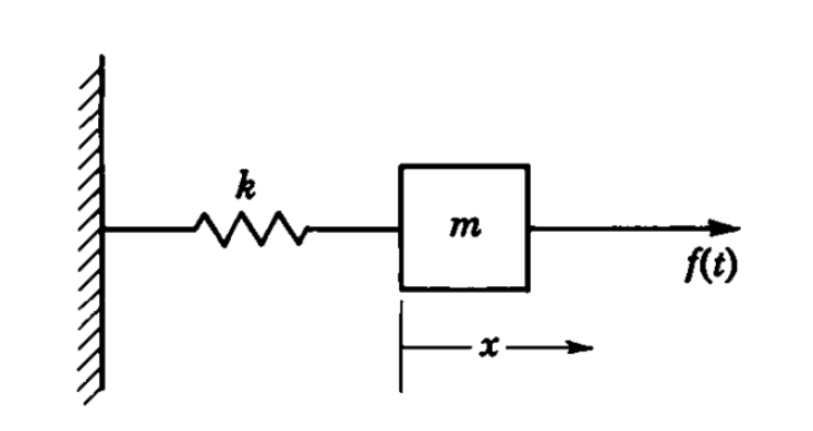
vibration model

Forced vibration:

md2xdt2+kx=f(t)x(0)=dx(0)dt=0ms2x¯+kx¯=f¯.

Thus, if we write

ω02=km,

the transform of the required solution is

x¯=1mf¯s2+ω02.

Since 1s2+ω02 is the transform of sin⁡ω0tω0, this product can be considered as the product of the transforms of sin⁡ω0tmω0 and f(t), and hence use of the convolution (T10) gives the solution

x=1mω0∫0tf(u)sin⁡ω0(t−u) du

in terms of an arbitrary force function f(t).

Example4: Solving the ODEs with Laplace Transform ​

We require the solution of the simultaneous equations

dxdt−y=etdydt+x=sin⁡t}

which satisfies the conditions

x(0)=1,y(0)=0.

The transforms of equations satisfying initial conditions are

sx¯−y¯=1s−1+1x¯+sy¯=1s2+1}

from which we obtain, algebraically,

x¯=s(s−1)(s2+1)+ss2+1+1(s2+1)2y¯=−1(s−1)(s2+1)−1s2+1+s(s2+1)2

If the first terms on the right-hand sides of these equations are expanded in partial fractions, there follows

x¯=12[1s−1+1s2+1+ss2+1+2(s2+1)2]y¯=12[−1s−1−1s2+1+ss2+1+2s(s2+1)2]}

and reference to Table 1 gives the required solution,

x=12(et+2sin⁡t+cos⁡t−tcos⁡t)y=12(−et−sin⁡t+cos⁡t+tsin⁡t)}.

Laplace Transform: Beyond solving ODEs ​

The physical significance of Laplace Transform (LT): from time domain s(t) to frequency domain S(ω)

HW ​

Question 1 ​

Q1: Find the Laplace transform of the following functions (10 marks)

1.1t3,1.2d3fdt3

Answer:

1.1 At first, it's known that with L 'Hopital's Law:

limt→∞tnest→limt→∞ntn−1sest→⋯→limt→∞n!snest=0L{t3}=∫0∞t3e−st dt=−1s∫0∞t3 d(e−st)=−1s(t3e−st|0∞−∫0∞3t2e−st dt)=1s∫0∞3t2e−st dt=−1s2∫0∞3t2 d(e−st)=−1s2(3t2e−st|0∞−∫0∞6te−st dt)=1s2∫0∞6te−st dt=−1s3∫0∞6t d(e−st)=−1s3(6te−st|0∞−∫0∞6e−st dt)=1s3∫0∞6e−st dt=−6s4∫0∞e−st d(−st)=−6s4e−st|0∞=6s4,s>0.

1.2: Assume the function f(t),dfdt,d2fdt2 is of exponential order, dfdt,d2fdt2,d3fdt3. Then as t→∞,e−stf(t),e−stdfdt,e−std2fdt2 vanishes.

L{d3fdt3}=∫0∞e−std3fdt3 dt=∫0∞e−stddt(d2fdt2) dt=e−std2fdt2|0∞+s∫0∞d2fdt2e−st dt=−d2f(0+)dt2+s∫0∞e−stddt(dfdt) dt=−d2f(0+)dt2+s(e−stdfdt|0∞+s∫0∞dfdte−st dt)=−d2f(0+)dt2−sdf(0+)dt+s2∫0∞e−stdfdt dt=−d2f(0+)dt2−sdf(0+)dt+s2(e−stf(t)|0∞+s∫0∞f(t)e−st dt)=−d2f(0+)dt2−sdf(0+)dt−s2f(0+)+s3L{f(t)}.

Question2 ​

Q2: Solve the following problem using Laplace transform (10 marks)

dydx+ky=0,y(0)=1.

Answer: Assume y is of exponential order. Then using Laplace transform at both sides, then

dydx=−ky⟹L{dydx}=L{−ky}∫0∞e−sxdydx dx=−k∫0∞e−sxy(x) dxe−sxy(x)|0∞+s∫0∞e−sxy(x) dt=−k∫0∞e−sxy(x) dx(s+k)∫0∞e−sxy(x) dx=−e−sxy(x)|0∞=y(0)=1⟹∫0∞e−sxy(x) dx=1s+k,s≠−k.

Since L{e−ax}=1/(s+a), then using inverse of laplace transform:

y(x)=L−1{1s+k}=e−kx

And e−kx is exactly of exponential order, then problem solved.

Released under the MIT License.