Skip to content

Angle Rigidity applied in Multiagent Formation Control [1] ​

1. 2D ​

To achieve a planar formation by a group of mobile robots, many formation control algorithms have been designed, most of which require the measurement of relative positions[2], or aligned bearings, or communication. In [2], a gradient-based formation stabilization control law is designed to achieve an infinitesimally angle rigid formation, in which the measurements of relative position and wireless communication of neighbors' angle error information are both needed. In this section, we demonstrate how to stabilize a multiagent planar formation using only local angle measurements with the help of the angle rigidity theory.

For an agent i moving in the plane, we consider its dynamics are governed by single-integrator

(1.1)p˙i=ui,i=1,…,N

where pi∈R2 denotes agent i 's position, ui∈R2 is the control input to be designed, and N is the number of agents in the group. Agent i can only measure angles; to be more specific, it can only measure the angle ϕij∈[0,2π) with respect to another agent j evaluated counter-clockwise from the X-axis of its own local coordinate frame of choice that is fixed to the ground.

To avoid confusion in the stability analysis, we first describe all variables in a global coordinate frame and finally we demonstrate that this global coordinate frame is unnecessary. Now we define the bearing gij∈R2 to be the unit vector pointing from agent i to j, i.e.,

gij=pj−pi‖pj−pi‖=[cos⁡ϕijsin⁡ϕij]

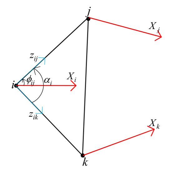
where ϕij determines uniquely gij when pi≠pj. Therefore, when ϕij can be measured, gij is known. In the triangle △ijk shown in Figure 1.1, the interior angle αi can be computed by

αi=∡kij=arccos⁡(gij⊤gik)

using bearings gij and gik. Note that the X-axes of agents i,j, and k do not need to align, and the angle to be controlled is not the measured angle ϕij, but the relative angle αi.

Measurement
Figure 1.1: Agent i 's angle measurements.
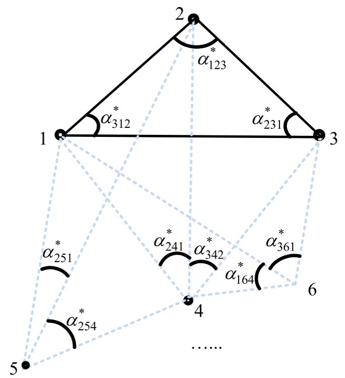
Formation
Figure 1.2: Constructing desired formation by using Case 3 of Type-I vertex addition starting from △ 123.

We construct the desired planar formation through a sequence of Type-I vertex additions (Case 3) from a generically angle rigid 3-vertex angularity, which is globally angle rigid according to Proposition 1 in angle rigidity. First, in an N-agent formation, we label the agents by 1∼N. Then, agents 1,2 , and 3 aim at forming the first triangular shape, and each of agents 4∼N aims at achieving two desired angles formed with other three agents (see Figure 1.2). By repeatedly adding new agents through the Type-I vertex addition operation, the aim is to achieve the desired angle rigid formation specified as follows. For agents 1−3

(1.2)limt→∞e1(t)=limt→∞(α312(t)−α312∗)=0(1.3)limt→∞e2(t)=limt→∞(α123(t)−α123∗)=0(1.4)limt→∞e3(t)=limt→∞(α231(t)−α231∗)=0

where αjik∗∈(0,π),i,j,k∈{1,2,3} denote agent i 's desired angle formed with agents j,k. For agents 4−N

(1.5)limt→∞ei1(t)=limt→∞(αj1ij2(t)−αj1ij2∗)=0(1.6)limt→∞ei2(t)=limt→∞(αj2ij3(t)−αj2ij3∗)=0

where i=4,…,N,j1<i,j2<i,j3<i, and αj1ij2∗∈(0,π),αj2ij3∗∈(0,π) denote agent i 's two desired angles formed with agents j1,j2,j3∈{1,2,…,i−1},j1≠j2≠j3. Therefore, the angle-only formation control problem to be solved in this section is formally described below.

Problem 1

Given feasible desired angles fA={α312∗,α123∗,α231∗,α241∗,α342∗,…,αi1Ni2∗,αi2Ni3∗}, design control law ui by only using angle measurements ϕij to achieve (1.2)-(1.6).

Remark 1.1

One may also choose other cases in Type-I and Type-II vertex addition operations to construct the desired formations. However, the constructed formations are not globally angle rigid or the realization depends on the knowledge of the neighbors' angle error, which are the drawbacks of the other cases when they are applied to formation control. For example, in Case 1 of Type-II vertex addition [Figure 4(d) in angle rigidity], Proposition 2 in angle rigidity shows that the constructed formation is only angle rigid which may cause ambiguity; moreover, the angle αk1j1i cannot be obtained by agent i 's local angle measurements.

A. Triangular Formation Control for Agents 1-3 ​

To achieve the desired angles for agents 1−3, we design their formation control laws

(1.7)ui=−(αi−αi∗)(gi(i+1)+gi(i−1))

where i∈{1,2,3},gi(i+1)=g31 when i=3 and gi(i−1)=g13 when i=1, and αi represents α(i−1)i(i+1) for conciseness.

To obtain the convergence of the angle errors, we first analyze the dynamics of the angle errors ei(t),i=1,2,3. We use the dot product of two bearings to obtain the angle error dynamics. According to (1.2) in angle rigidity, agent 1's angle error dynamics can be obtained by

α˙1=−[Pg13d13sin⁡α1(p˙3−p˙1)]⊤g12−g13⊤Pg12d12sin⁡α1(p˙2−p˙1).

By following the calculation in Appendix A (TODO), one has the first three agents' angle error dynamics

e˙f=[α˙1α˙2α˙3]⊤=F(ef)ef(1.8)=[−z1f12f13f21−z2f23f31f32−z3][α1−α1∗α2−α2∗α3−α3∗]

where ef=[α1−α1∗α2−α2∗α3−α3∗]⊤,zi=(sin⁡αi)(1/di(i+1)+1/di(i−1)),fij=(sin⁡αj)/dij.

To guarantee that the triangular formation system under the control law (1.7) is well defined, we first prove that no collinearity and collision will take place under (1.8) if the formation is not collinear initially.

Lemma 1.1 (No collinearity)

For the three-agent formation, if the initial formation is not collinear, it will not become collinear for t>0 under the angle error dynamics (1.8).

Proof:

Proof of Lemma 1.1

Consider the manifold Ma={(α1, α2,α3)∣α1+α2+α3=π,0<α1<π,0<α2<π, and 0<α3<π} which is an open set. To show Ma is positively invariant, we show that for any (α1,α2,α3)∈Ma it is impossible for αi,i=1,2,3 to escape Ma under (1.8). Consider the boundary states αi(t)=π−ε1 with ε1=0+, αi+1(t)=ε2=0+,αi−1(t)=ε3=0+,ε1=ε2+ε3.

According to (1.8), one has

e˙i=−ziei+fi(i+1)ei+1+fi(i−1)ei−1

Since 0<αi∗<π and αi∗ is bounded away from 0 and π, one has

ziei=zi(αi−αi∗)>0fi(i+1)ei+1=fi(i+1)(αi+1−αi+1∗)<0fi(i−1)ei−1=fi(i−1)(αi−1−αi−1∗)<0

which implies that e˙i(t)<0. Thus, when αi(t) is close to π,αi(t) will decrease, which implies that Ma is positively invariant, i.e., trajectories starting from Ma remains in Ma. Q.E.D.

◻

Lemma 1.2 (No collision)

For the three-agent formation, if the initial angles αi(0)≠0,i=1,2,3, no collision will take place for t>0 under the formation control law (1.7).

Proof:

Proof of Lemma 1.2

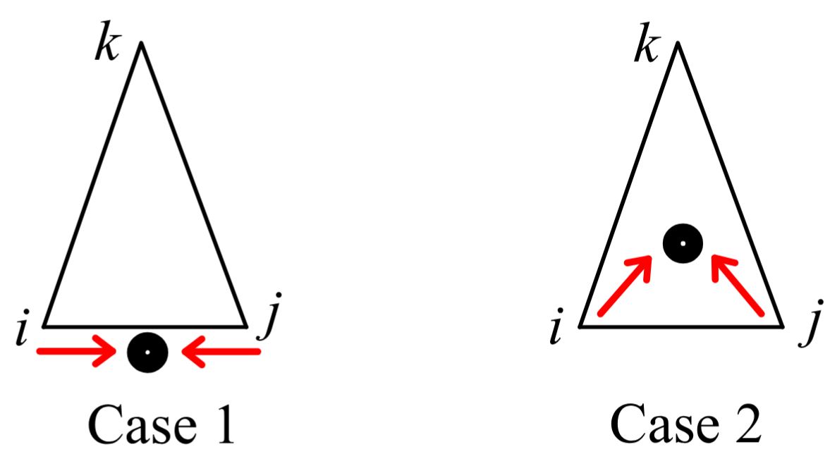
Suppose on the contrary that collision may happen between agents i and j at t=t1. Then, one of the following two cases shown in Figure 1.3 will take place.

For the first case, p˙i(t1)=−γp˙j(t1), where γ is a positive constant. Note that the moving direction of agent i under the control law (1.7) is always the bisector of the interior angle αi. According to Lemma 1.1, no collinearity will happen for t>0 which implies that gik(t)≠−gjk(t) for t>0. According to the control law (1.7), p˙i(t1)=−γp˙j(t1) requires gik(t1)=−gjk(t1), which is impossible for t>0.

For the second case, since agents i and j move toward the inside of the triangle, it follows from the control law (1.7) that π2−ε1=αi(t1−)<αi∗ and π2−ε2=αj(t1−)<αj∗, where ε1=0+and ε2=0+. Then, αi∗+αj∗+αk∗=π>π+αk∗−ε1−ε2, which contradicts the fact that αk∗ is bounded away from 0. Q.E.D.

◻

Case
Figure 1.3: Collision cases.

Now, we give the main result for the convergence of the triangular formation.

Theorem 1 (Stability of the first three agents)

For the triangular formation under the control law (1.7), if αi(0)≠0 and the initial angle errors ei(0),i=1,2,3 are sufficiently small, the angle errors ei and agents' control input ui(t) converge exponentially to zero.

Proof:

Proof of Theorem 1

From Lemmas 1.1 and 1.2, no collinearity and collision will take place since sin⁡αi≠0,dij≠0,∀i,j=1,2,3, which guarantees that the closed-loop system under the control law (1.7) is well defined. Since e1+e2+e3=∑i=13αi−∑i=13αi∗≡ 0 , the angle error dynamics (1.8) can be reduced to

(1.9)e˙s=[e˙1e˙2]=[−(z1+f13)f12−f13f21−f23−(z2+f23)][e1e2]=Fs(es)es.

Let U2∈R2 denote a neighborhood of the origin {e1=e2=0}, in which we investigate the local stability of (1.9). Linearizing (1.9) around the origin, we obtain

(1.10)e˙s=L1(α∗)es

where L1(α∗)=Fs(es)|es=0. Then, one has

(1.11)tr(L1(α∗))=−z1∗−f13∗−z2∗−f23∗<0

\begin{aligned} \operatorname{det}\left(L_{1}\left(\alpha^{*}\right)\right)&=\left(z_{1}^{*}+f_{13}^{*}\right)\left(z_{2}^{*}+f_{23}^{*}\right)-\left(f_{21}^{*}-f_{23}^{*}\right)\left(f_{12}^{*}-f_{13}^{*}\right)\\ &>z_{1}^{*} f_{23}^{*}+z_{2}^{*} f_{13}^{*}+f_{21}^{*} f_{13}^{*}+f_{12}^{*} f_{23}^{*}>0 \tag{1.12} \end{aligned}

where zi∗=zi|es=0,fij∗=fij|es=0, and tr() and det() denote the trace and determinant of a square matrix, respectively, and we have used z1∗z2∗>f21∗f12∗. According to (1.11) and (1.12), one has that L1(α∗) is Hurwitz. According to the Lyapunov Theorem, there always exists positive definite matrices P1∈R2×2 and Q1∈R2×2 such that −Q1=P1L1(α∗)+L1⊤(α∗)P1. Design the Lyapunov function candidate as

V1=es⊤P1es

Taking the time-derivative of V1 yields

V˙1=−es⊤Q1es⩽−λmin(Q1)λmax(P1)V1

which implies that V1(t)⩽V1(0)e−λmin (Q1)λmax (P1)t where λmax  and λmin  denote the maximum and minimum eigenvalues of a real symmetric matrix, respectively. Since P1>0, one has

(1.12)e12+e22=‖es‖2⩽V1λmin(P1)⩽V1(0)λmin(P1)e−λmin(Q1)λmax(P1)t

Also, one has

e32=e12+e22+2e1e2⩽2(e12+e22)⩽2V1(0)λmin(P1)e−λmin(Q1)λmax(P1)t

which implies that ei under the dynamics (1.8) is exponentially stable when the initial states lie in U2. According to (1.7), ‖ui‖⩽2|ei| also converge to zero at an exponential rate, which implies that pi,i=1,2,3 will converge to fixed points and the orientation and scale of the formation will then be fixed. Q.E.D.

◻

Remark 1.2

With noncollinear initial positions, the first three agents' angle error dynamics e˙s=Fs(es)es are globally stable, as a consequence of the Poincare-Bendixson theorem employed in [34, Theorem 6]. The difference between the angle error dynamics e˙s=Fs(es)es and the dynamics given in [34] is that sin⁡αi shown in zi,fij in (1.8) is replaced by sin⁡αi2 in [34]. However, for a triangular formation, it holds that sin⁡αi2>0 and sin⁡αi>0 for all αi∈(0,π). Therefore, one can similarly obtain the almost global stability of e˙s=Fs(es)es by following [34, Th. 6].

After proving that the first three agents converge to the desired formation, we now look at the remaining agents.

B. Adding Agents 4 to N in Sequence ​

In this subsection, we consider that agent i,i=4,…,N, are added to the formation through the Type-I vertex addition operation with two desired angles. For agents i=4,…,N, the control algorithm is designed to be

ui=−(αj1ij2−αj1ij2∗)(gij1+gij2)(1.13)−(αj2ij3−αj2ij3∗)(gij2+gij3)

where αj1ij2∗∈(0,π) and αj2ij3∗∈(0,π),j1<i,j2<i,j3<i,j1≠j2≠j3 are the two desired angles. Different from the first three agents, the bearing measurement topology from agents 4 to N becomes directed.

To prove the stability from agents 4 to N, we use induction. Toward this end, we need to first prove that the 4 -agent formation of 1−4 converges to the desired shape exponentially. For the 4 -agent formation, the control algorithm (1.13) can be written as

u4=−(α241−α241∗)(g41+g42)(1.14)−(α342−α342∗)(g42+g43).

Then, one has the following result.

Lemma 1.3 (Stability of agent 4):

Suppose ei(0),i=1,2,3 are sufficiently small and the subformation of 1,2 , and 3 is governed by (1.7). Under the control algorithm (1.14) for agent 4 , if the initial distances d4i(0) are sufficiently bounded away from zero, the initial angle errors e41(0) and e42(0) are sufficiently small and α341∗=α241∗+α342∗,sin⁡α124∗>sin⁡α412∗,sin⁡α423∗>sin⁡α234∗, then e41(t) and e42(t) converges to zero exponentially.

Proof:

Proof of Lemma 1.3

To analyze the stability of the angle errors e41 and e42 under the control algorithm (1.14), we first calculate the angle error dynamics of e41 and e42. According to the calculation in Appendix B (TODO), one has the following angle error dynamics:

e˙4=[α˙241α˙342]⊤=F4(e4)e4+W(e4)es(1.15)=[j11j12j21j22][e41e42]+[w11w12w21w22][e1e2]

where j11=−sin⁡α241d41−sin⁡α241d42,j22=−sin⁡α342d43−sin⁡α342d42,j12=−(sin⁡α241)+(sin⁡α341)d41+sin⁡α342d42,j21=−(sin⁡α342)+(sin⁡α341)d43+sin⁡α241d42,w11=g42⊤Pg41(g12+g13)d41sin⁡α241, w12=g41⊤Pg42(g21+g23)d42sin⁡α241,w21=−g42⊤Pg43(g31+g32)d43sin⁡α342,w22=g43⊤Pg42(g21+g23)d42sin⁡α342−g42⊤Pg43(g31+g32)d43sin⁡α342.

Now, by conducting linearization towards (1.15) in a small neighborhood of the origin {e1=0,e2=0,e41=0,e42=0}, one has

(1.16)e˙4=L2(α∗)e4+W¯es

where L2(α∗)=F4(e4)|es=0,e4=0 and W¯=W(e4)|es=0,e4=0. Then, one has

tr(L2(α∗))=(j11+j22)|es=0,e4=0<0det(L2(α∗))=(j11j22−j12j21)|es=0,e4=0=d41∗(sin⁡α241∗sin⁡α342∗+sin2⁡α342∗+sin⁡α342∗sin⁡α341∗)d41∗d42∗d43∗+d43∗(sin⁡α241∗sin⁡α342∗+sin2⁡α241∗+sin⁡α241∗sin⁡α341∗)d42∗d41∗d43∗−d42∗(sin⁡α241∗sin⁡α341∗+sin⁡α341∗sin⁡α342∗+sin2⁡α341∗)d41∗d42∗d43∗

where dij∗ is the distance between agents i and j in the desired formation. Therefore, if det(L2(α∗))>0, one has that L2(α∗) is Hurwitz. By using the law of Sines, sin⁡α124∗>sin⁡α412∗ and sin⁡α423∗>sin⁡α234∗ imply d41∗>d42∗ and d43∗>d42∗, respectively. Then, one can check that det(L2(α∗))>0 if d41∗>d42∗ and d43∗>d42∗ hold because, on the one hand

d43∗sin⁡α241∗sin⁡α341∗>d42∗sin⁡α241∗sin⁡α341∗d41∗sin⁡α341∗sin⁡α342∗>d42∗sin⁡α341∗sin⁡α342∗

and, on the other hand

sin2⁡α341∗=[sin⁡α241∗cos⁡α342∗+cos⁡α241∗sin⁡α342∗]2=sin2⁡α241∗cos2⁡α342∗+cos2⁡α241∗sin2⁡α342∗+2sin⁡α241∗cos⁡α342∗cos⁡α241∗sin⁡α342∗

and d41∗sin2⁡α342∗>d42∗sin2⁡α342∗cos2⁡α241∗,d43∗sin2⁡α241∗>d42∗sin2⁡α241∗cos2⁡α342∗ and d41∗sin⁡α241∗sin⁡α342∗+d43∗sin⁡α241∗sin⁡α342∗>2d42∗sin⁡α241∗sin⁡α342∗>2d42∗sin⁡α241∗cos⁡α342∗cos⁡α241∗sin⁡α342∗. By combining (1.10) and (1.16) together, one has the overall linearized 4-agent angle error dynamics

(1.17)e¯˙4=[e˙se˙4]=L4(α∗)e¯4=[L1(α∗)0W¯L2(α∗)][ese4]

When L1(α∗) and L2(α∗) are Hurwitz, one has that L4(α∗) is also Hurwitz. When L4(α∗) is Hurwitz, for an arbitrary positive definite matrix Q2∈R4×4, there always exists positive definite matrix P2∈R4×4 such that −Q2=P2L4(α∗)+L4⊤(α∗)P2. Design the Lyapunov function candidate as

V2=e¯4⊤P2e¯4.

Taking the time-derivative of V2 along (1.17) yields

(1.18)V˙2=−e¯4⊤Q2e¯4⩽−λmin(Q2)‖e¯4‖2⩽−λmin(Q2)λmax(P2)V2

Then, one has

(1.19)‖e4‖2⩽‖e¯4‖2⩽V2λmin(P2)⩽V2(0)λmin(P2)e−(λmin(Q2)λmax(P2))t.

which implies that the agent 4's angle error e4 also converges to zero at an exponential rate. To guarantee that ‖W(e4)‖ is bounded and control law (1.14) is well defined, the collision between agent 4 and agents 1−3 should be avoided. Taking agent 1 as an example, one has

‖p4(t)−p1(t)‖=‖p4(0)+∫0tu4(s)ds−p1(0)−∫0tu1(s)ds‖⩾‖p4(0)−p1(0)‖−∫0t‖u1(s)−u4(s)‖ds⩾d14(0)−2∫0t(|e1(s)|+|e41(s)|+|e42(s)|)ds

Since d14(0) is sufficiently bounded away from zero, there always exists a finite time T such that in the time interval [0,T], there is no collision between agent 4 and agent 1 . Then, according to (1.12) and (1.19), one has

‖p4(T)−p1(T)‖⩾d14(0)−2∫0⊤(|e1(s)|+|e41(s)|+|e42(s)|)ds⩾d14(0)−4[λmax(P1)λmin(Q1)V1(0)λmin(P1)(1−e−λmin(Q1)2λmax(P1)T)+λmax(P2)λmin(Q2)2V2(0)λmin(P2)(1−e−(λmin(Q2)2λmax(P2)T)]

where we have used the fact that |e41|+|e42|⩽2(e412+e422)=2‖e4‖. Since V1(0) and V2(0) are sufficiently small and d14(0) is sufficiently bounded away from zero, one has ‖p4(T)−p1(T)‖>0 since d14(0)>4[λmax (P1)λmin (Q1)V1(0)λmin (P1)+λmax (P2)λmin (Q2)2V2(0)λmin (P2)]. Then, we extend T to infinity. Because e−λmin(Q1)2λmax(P1)t>0 and e−(λmin(Q2)2λmax(P2))t>0,∀t>0, one has that d41(t)=‖p4(t)−p1(t)‖>0 for t>0. On the other hand, since the initial angle errors e41(0) and e42(0) are sufficiently small and e1(t),e2(t),e41(t) and e42(t) converge at an exponential speed, α241(t) and α342(t) will be bounded away from 0 and π. Therefore, ‖W(e4)‖ is bounded and (1.15) is well defined. The proof for 4 -agent formation is completed.

Now, we present the main result for agents 4 to N.

Theorem 2 (Stability of all the agents)

Consider a formation of N>3 agents, each of which is governed by (1.1). Suppose ei(0),i=1,2,3 are sufficiently small and the subformation of 1,2,3 is governed by (1.7). For agent i,4⩽i⩽N, if the initial distances dij1(0),dij2(0), and dij3(0) are sufficiently bounded away from zero, the initial angle errors ei1(0) and ei2(0) are sufficiently small and αj3ij1∗=αj2ij1∗+αj3ij2∗,sin⁡αj1j2i∗>sin⁡αij1j2∗,sin⁡αij2j3∗>sin⁡αj2j3i∗, then under (1.13), the formation achieves its desired shape exponentially.

Proof:

Details of Proof

From Lemma 1.3, 4-agent formation achieves the desired shape exponentially. Suppose for a 4<k<N, the k-agent formation converges to the desired shape exponentially. We need to prove that for (k+1)-agent formation, the relative angle errors e(k+1)1=αj1(k+1)j2−αj1(k+1)j2∗ and e(k+1)2=αj2(k+1)j3−αj2(k+1)j3∗ converge to zero exponentially. Similar to the proof from (1.14) to (1.18), one has that the angle errors e(k+1)1 and e(k+1)2 exponentially converge to zero. Therefore, the control algorithm (1.13) can locally stabilize the agent k+1, i.e., the ( k+1 )-agent formation converges to the desired shape exponentially. So, from induction, N-agent formation converges to the desired formation shape exponentially. Q.E.D.

◻

Remark 1.3

Note that the control laws (1.7) and (1.13) can be described by a unified form

(1.20)ui=−∑(j,i,k)∈A(αjik−αjik∗)(gij+gik)

where A={(1,2,3),(2,3,1),(3,1,2),(1,4,2),(2,4,3),…, (j1,k,j2),(j2,k,j3),…,(i1,N,i2),(i2,N,i3)},j1<k,j2<k,j3<k,j1≠j2≠j3. Therefore, the unified control algorithm (1.20) can locally stabilize the angle rigid formation constructed through a sequence of Type-I vertex additions (Case 3) from a triangular shape. Because we aim at obtaining local stability for multiagent formations, we only consider the range of the desired angles belonging to ( 0,π ) in (1.2)-(1.6), and the case of αi(0)∈(π,2π),αi∗∈(π,2π) can be similarly obtained. However, to achieve a general infinitesimally and minimally angle rigid formation, one can use the gradient-based control law

p˙=u=−(∂V3∂p)⊤=−RA⊤(p)(α−α∗)

where V3=0.5(α−α∗)⊤(α−α∗),p,u,α are the stack vectors of pi,ui,αjik, respectively. It follows that V˙3=−(α−α∗)⊤RA(p)RA⊤(p)(α−α∗). Because RA(p)RA⊤(p) is positive definite when p is in a small neighborhood of the desired formation, one has the local convergence of (α−α∗).

Remark 1.4

Although each agent's position in (1.1) is described in the global coordinate frame, it is not required in the implementation of control algorithm (1.20). The control algorithm (1.20) can be realized in each agent's local coordinate frame since (1.20) can be equivalently written in agent i 's local coordinate frame

(1.21)Rgbui=−∑(j,i,k)∈A(αjik−αjik∗)Rgb(gij+gik)

where Rgb∈SO(2) is the rotation matrix from the global coordinate frame to agent i 's local coordinate frame, Rgbui is the controller input in agent i 's local coordinate frame, and Rgbgij,Rgbgik are the local bearings measured in agent i 's local coordinate frame. Since (αjik−αjik∗) is a scalar and αjik is the same under different coordinate frames, (1.21) and (1.20) are equivalent.

Reference ​

  1. Liangming Chen, Ming Cao and Chuanjiang Li, Angle rigidity and its usage to stabilize multiagent formations in 2-D, IEEE Trans. Autom. Control, vol. 66, no. 8, pp. 3667–3681, Aug. 2021: Section IV. Note that z is replaced by g for bearing.
  2. Gangshan Jing, G. Zhang, H. W. J. Lee, and L. Wang, Angle-based shape determination theory of planar graphs with application to formation stabilization, Automatica J. IFAC, vol. 105, pp. 117–129, Jul. 2019: arXiv.

Released under the MIT License.