Introduction of Linear algebra

This is the note from MNE8108 Engineering Methods in the Department of Mechanical Engineering, CityU (semester A, 2025)

Contents mostly From Linear Algebra by Arnold J. Insel etc.

Appendix A: Sets

Definitions

Definition: sets

collection of objects, called elements of the set

• $x\in A;x\notin A$
• list them using $\{\}$
• no order: $\{1,2\}=\{2,1\}$
  

subsets:

• $B\subseteq A$
• proper set: $B\subseteq A,B\ne A$
• empty set: $\varphi$

calculation

• union: $A\cup B$

• intersection: $A\cap B$

  • disjoint sets: $A\cap B=\varphi$

• finite sets: $\{1,2\}$

• infinite sets: $\mathbb{R}$

Number systems:

• Natural number: $\mathbb{N}({\mathbb{N}}_0:(\text{ include }0);{\mathbb{N}}_1:(\text{ not include }0))$
• Integral number: $\mathbb{Z}$
• Rational number: $\mathbb{Q}$
• Real number: $\mathbb{R}$
• Complex number: $\mathbb{C}$

Cardinal number: the number if elements of a set

For infinite sets:

• Countable sets: ${\text{alef}}_0$: $\mathbb{N},\mathbb{Z},\mathbb{Q}$
• Uncountable sets: beth one: $\mathbb{R},\mathbb{C}$

operations

operation: from a set to itself

Unary:

• negation: $-$
• factorial: $!$
• trigonometric: $\sin ,\cos ,\cdots$

Binary:

• $+-x/$

tenary: ...

Arithmetic

• $+,\times$

  Set	${\mathbb{N}}_0$	${\mathbb{N}}_1$
  Elements	$\mathbf{0},1,2,3\in {\mathbb{N}}_0$	$1,2,3,4\in {\mathbb{N}}_1$
  Operation	$+$	$\times$
  Closure	$1+2=3\in {\mathbb{N}}_0$	$2\times 3=6\in {\mathbb{N}}_1$
  Associative	$(1+2)+3=1+(2+3)$	$(2\times 3)\times 4=2\times (3\times 4)$
  Commutative	$1+2=2+1$	$2\times 3=3\times 2$
  Distributive	-	-

• $-,/$

  Set	$\mathbb{Z}$	$\mathbb{Q}$
  Elements	$x,y,\cdots \in \mathbb{Z}$	$x,y\cdots \in \mathbb{Q}$
  Operation	$+$	$\times$
  Identity	$0$	$1$
  inverses	$-x$	$\frac{1}{x}$ or $x^{-1}$

More generally:

Set	$S$	$\mathbb{Z}$	$\mathbb{Q}$
Elements	$x,y,z,\cdots \in S$	$x,y,z,\cdots \in \mathbb{Z}$	$x,y,z,\cdots \in \mathbb{Q}$
Operation	$\ast$	$+$	$\times$
Closure	$x\ast y\in S$	$x+y\in \mathbb{Z}$	$x\times y\in \mathbb{Q}$
Associative	$(x\ast y)\ast z=x\ast (y\ast z)$	$(x+y)+z=x+(y+z)$	$(x\times y)\times z=x\times (y\times z)$
Commutative	$x\ast y=y\ast x$	$x+y=y+x$	$x\times y=y\times x$
Distributive	-	-	-
Identity	$\mathrm{\exists }e\in S:x\ast e=e\ast x=x$	$0$	$1$
inverses	$\mathrm{\forall }x,\mathrm{\exists }{x}^{-1}\in S:x\ast x^{-1}=x^{-1}\ast x=e$	$-x$	$\frac{1}{x}$ or $x^{-1}$

group

Given:

• Set of elements $G$
• Operation: $\ast$

Set	$G$
Elements	$x,y,z,\cdots \in G$
Operation	$\ast$
Closure	$x\ast y\in G$
Associative	$(x\ast y)\ast z=x\ast (y\ast z)$
Commutative	$x\ast y=y\ast x$? (Not requestes)
Distributive	-
Identity	$\mathrm{\exists }e\in G:x\ast e=e\ast x=x$
inverses	$\mathrm{\forall }x,\mathrm{\exists }{x}^{-1}\in G:x\ast x^{-1}=x^{-1}\ast x=e$

• If communtative: commutative group / abelian group
• If not commutative: non-commutative group / non-abelian group

Example of group:

• commutative:

  • $\mathbb{Z}$ with $+$
  • $\mathbb{Z}$ commutes under $+$

• non-commutative:

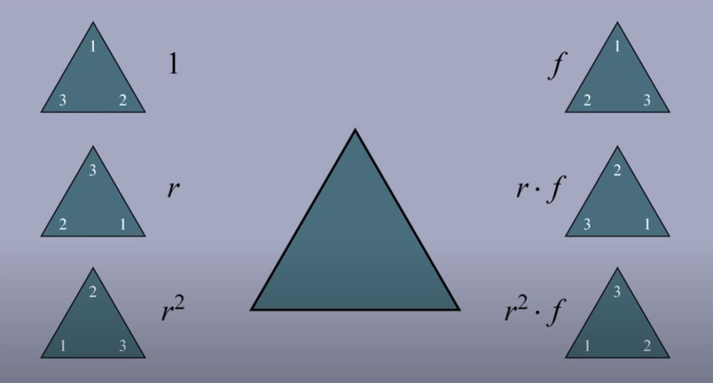
  • Dihedral group:
    • $r$: rotation
    • $f$: reflection
    • $r\cdot f\ne f\cdot r$
  

Ring

Given:

• Set of elements $R$
• Operation: $+,\times$

Set	$R$
Elements	$a,b,c,\cdots \in R$
Operation	Addition $+$	Multiplication $\times$
Closure	$a+b\in R$	$a\times b\in R$
Associative	$(a+b)+c=a+(b+c)$	$(a\times b)\times c=a\times (b\times c)$
Commutative	$a+b=b+a$	$a\times b=b\times a$? (Not required)
Distributive	$a\times (b+c)=a\times b+a\times c$; $(b+c)\times a=b\times a+c\times a$
Identity	$\mathrm{\exists }0\in R:a+0=0+a=a$	$\mathrm{\exists }1\in R:1\times a=a\times 1=a$
Inverses	$\mathrm{\exists }(-a)\in R:a+(-a)=0$	$\mathrm{\exists }{a}^{-1}\in R$? (Not required)

• distributive: left distributive v.s. right distributive
• If communitative, just check one distributivity

Example of ring:

• commutative:
  • $\mathbb{Z}$ with $+,\times$
• non-commutative:
  • $M_2(R)$ with matrix addition and matrix multiplication

Appendix C: Fields

Given:

• Set of elements $F$
• Operation: $+,\times$

Set	$F$
Elements	$a,b,c,\cdots \in F$
Operation	Addition $+$
Closure	$a+b\in F$
Associative	$(a+b)+c=a+(b+c)$
Commutative	$a+b=b+a$
Distributive	$a\times (b+c)=a\times b+a\times c$
Identity	$\mathrm{\exists }0\in F:a+0=0+a=a$
inverses	$\mathrm{\exists }(-a)\in F:a+(-a)=0$

Example of field:

• $\mathbb{Q}$ with $+,\times$
• $\mathbb{R}$ with $+,\times$
• $\mathbb{C}$ with $+,\times$
• $\mathrm{GF}(2)/Z_2$, a finite field with two elements(0,1); operations: XOR + AND.

Modulo Arithmetic:

• $17(\mathrm{mod}5)=2$
• $17\equiv 2(\mathrm{mod}5)$

Theorem C.1 (Cancellation Laws)

$\mathrm{\forall }a,b,c$ in a field, the following statements are true:

• If $a+b=c+b$, then $a=c$
• If $a\cdot b=c\cdot b,b\ne 0$, then $a=c$

Corollary

the identity elements and the inverse elements are unique

Theorem C.2

$\mathrm{\forall }a,b$ in a field, the following statements are true:

• $a\cdot 0=0$
• $(-a)\cdot b=a\cdot (-b)=-(a\cdot b)$
• $(-a)\cdot (-b)=a\cdot b$

1.2 vector space

Given:

• Set of elements $V,F$
• Operation: $+,\times$
• Commutative group $V$ under $+$, with a Field $F$

Set	$V$	$V$ and $F$	$F$	$F$
Elements	$\overrightarrow{u},\overrightarrow{v},\overrightarrow{w}\in V$		$a,b,c\in F$
Operation	Addition $+$	Scalar multiplication $\times$	Addition $+$	Multiplication $\times$
Closure	$\overrightarrow{u}+\overrightarrow{v}\in V$	$a\times \overrightarrow{u}\in V$	$a+b\in F$	$a\times b\in F$
Associative	$(\overrightarrow{u}+\overrightarrow{v})+\overrightarrow{w}=\overrightarrow{u}+(\overrightarrow{v}+\overrightarrow{w})$	$(a\times b)\times \overrightarrow{u}=a\times (b\times \overrightarrow{u})$	$(a+b)+c=a+(b+c)$	$(a\times b)\times c=a\times (b\times c)$
Commutative	$\overrightarrow{u}+\overrightarrow{v}=\overrightarrow{v}+\overrightarrow{u}$	$a\times \overrightarrow{u}=\overrightarrow{u}\times a$	$a+b=b+a$	$a\times b=b\times a$
Distributive	-	$a\times (\overrightarrow{u}+\overrightarrow{v})=a\times \overrightarrow{u}+a\times \overrightarrow{v};<br>(a+b)\times \overrightarrow{u}=a\times \overrightarrow{u}+b\times \overrightarrow{u}$	$a\times (b+c)=a\times b+a\times c$
Identity	$\mathrm{\exists }\overrightarrow{0}\in V:\overrightarrow{u}+\overrightarrow{0}=\overrightarrow{0}+\overrightarrow{u}=\overrightarrow{u}$	$1\times \overrightarrow{u}=\overrightarrow{u}$	$\mathrm{\exists }0\in F:a+0=0+a=a$	$\mathrm{\exists }1\in F:1\times a=a\times 1=a$
inverses	$\mathrm{\exists }(-\overrightarrow{u})\in V:\overrightarrow{u}+(-\overrightarrow{u})=\overrightarrow{0}$	$0\times u=\overrightarrow{0}$; $(-1)\times \overrightarrow{u}=-\overrightarrow{u}$	$\mathrm{\exists }(-a)\in F:a+(-a)=0$	$\mathrm{\exists }{a}^{-1}\in F:a\times a^{-1}=1$

Definition: vector space $\mathsf{V}$ [core]

A vector space $\mathsf{V}$ over a field $F$ consists of a set on which 2 operations (addition and scalar multiplication) are defined and closedness, s.t. the following conditions hold:

1. $\mathrm{\forall }x,y\in \mathsf{V},x+y=y+x$ (Commutativity of addition);
2. $\mathrm{\forall }x,y,z\in \mathsf{V},(x+y)+z=x+(y+z)$ (Associativity for each $x\in \mathsf{V}$);
3. There exists an element in $\mathsf{V}$ denoted by $0$ s.t. $x+0=0+x=x,\mathrm{\forall }x\in \mathsf{V}$;
4. $\mathrm{\forall }x\in \mathsf{V}$, there exists an element $y\in \mathsf{V}$, s.t. $x+y=0$;
5. $\mathrm{\forall }x\in \mathsf{V},1x=x$;
6. $\mathrm{\forall }a,b\in F,\mathrm{\forall }x\in \mathsf{V},(ab)x=a(bx)$;
7. $\mathrm{\forall }a\in F,\mathrm{\forall }x,y\in \mathsf{V},a(x+y)=ax+by$;
8. $\mathrm{\forall }a,b\in F,\mathrm{\forall }x\in \mathsf{V},(a+b)x=ax+bx$

Module definition: similar to vector space, but:

• commutative of scalar multiplication not required
• commutative of multiplication for number part, not required

Definition

• sum: $x+y$
• product: $ax$
• scalars: elements of $F$
• vectors: elements of vector space $\mathsf{V}$
• n-tuple: $n$ elements of a field in this form: $(a_1,\cdots ,a_n)$
  • entries / components: $a_1,\cdots ,a_n$
  • 2 n-tuples are equal if $a_i=b_i,\mathrm{\forall }i=0,1,2,\cdots ,n$
  • ${\mathsf{F}}^n$: set of all n-tuples with entries from a field $F$
  • vectors in ${\mathsf{F}}^n$: column vectors

Definition about some vector spaces

Definitions: Matrix

• diagonal entries: $a_{ij}$ with $i=j$
• i-th row: $a_{i1},a_{i2},\cdots ,a_{in}$
• j-th column: $a_{1j},a_{2j},\cdots ,a_{mj}$
• zero matrix: all zero
• square: the number of rows and columns are equal
• equal: $A_{ij}=B_{ij},\mathrm{\forall }1⩽i⩽m,1⩽j⩽n$
• set of all $m\times n$ matrices with entries from a field $F$ is a vector space: ${\mathsf{M}}_{m\times n}(F)$

matrix addition: $(A+B{)}_{ij}=A_{ij}+B_{ij}$ scalar multiplication: $(cA{)}_{ij}=c{A}_{ij}$

Definitions: function

Let $S$ be any nonempty set and $F$ be any field, and let $\mathcal{F}(S,F)$ denote the set of all functions from $S$ to $F$. Two functions $f$ and $g$ in $\mathcal{F}(S,F)$ are called equal if $f(s)=g(s)$ for each $s\in S$. The set $\mathcal{F}(S,F)$ is a vector space with the operations of addition and scalar multiplication defined for $f,g\in \mathcal{F}(S,F)$ and $c\in F$ by

$$(f+g)(s)=f(s)+g(s)\text{ and }(cf)(s)=c[f(s)]$$

for each $s\in S$. Note that these are the familiar operations of addition and scalar multiplication for functions used in algebra and calculus.

Definitions: polynominal

$$f(x)=a_n{x}^n+a_{n-1}{x}^{n-1}+\cdots +a_1{x}_1+a_0$$

• coefficient: $a_i,i=0,1,\cdots ,n$
• zero polynominal: $a_i=0,i=0,1,\cdots ,n$
• degree:
  • $-1$ for zero polynominal
  • largest exponent of $x$
• equal if equal degree and $a_i=b_i,i=0,1,\cdots ,n$

When $F$ is a field containing infinitely many scalars, we usually regard a polynomial with coefficients from $F$ as a function from $F$ into $F$

$$\begin{array}{rl}f(x)& =a_n{x}^n+a_{n-1}{x}^{n-1}+\cdots +a_1{x}_1+a_0\\ g(x)& =b_n{x}^n+b_{n-1}{x}^{n-1}+\cdots +b_1{x}_1+b_0\end{array}$$

addition and scalar multiplication:

$$\{\begin{array}{l}f(x)+g(x)=(a_n+b_n)x^n+(a_{n-1}+b_{n-1})x^{n-1}+\cdots +(a_0+b_0)\\ cf(x)=c{a}_n{x}^n+c{a}_{n-1}{x}^{n-1}+\cdots +c{a}_1{x}_1+c{a}_0\end{array}$$

set of all polynominal: $\mathsf{P}(F)$

Theorem 1.1: Cancellation Law for Vector Addition

If $x,y,z$ are vectors in a vector space, s.t. $x+z=y+z$, then $x=y$

Corolloary 1

The vector $\mathbf{0}$ is unique (zero vector)

Corolloary 2

The inverse element of vector is unique (additive inverse)

Theorem 1.2

In any vector space $\mathsf{V}$:

• $0\mathit{x}=\mathbf{0},\mathrm{\forall }\mathit{x}\in \mathsf{V}$
• $(-a)x=-(ax)=a(-x),\mathrm{\forall }a\in F,x\in \mathsf{V}$
• $a\mathbf{0}=\mathbf{0},\mathrm{\forall }a\in F$

1.3 subspace

Definition: subspace

A subset $\mathsf{W}$ of a vector space $\mathsf{V}$ over a field $F$ is called a subspace of $\mathsf{V}$ if $\mathsf{W}$ is a vector space over $F$ with the operations of addition and scalar multiplication defined on $\mathsf{V}$.

In any vector space $\mathsf{V}$, note that $\mathsf{V}$ and $\{0\}$ are subspaces. The latter is called the zero subspace of $\mathsf{V}$.

Theorem 1.3(subspace)[core]

Let $\mathsf{V}$ be a vector space and $\mathsf{W}$ a subset of $\mathsf{V}$. Then $\mathsf{W}$ is a subspace of $\mathsf{V}$ iff the following three conditions hold for the operations defined in $\mathsf{V}$.

• $0\in \mathsf{W}$.
• $x+y\in \mathsf{W}$ whenever $x\in \mathsf{W}$ and $y\in \mathsf{W}$.
• $cx\in \mathsf{W}$ whenever $c\in F$ and $x\in \mathsf{W}$.

Examples of subspaces

matrix

The transpose $A^t$ of an $m\times n$ matrix $A$ is the $n\times m$ matrix obtained from $A$ by interchanging the rows with the columns; that is, $(A^t{)}_{ij}=A_{ji}$.

A symmetric matrix is a matrix $A$ such that $A^t=A$.

• Clearly, a symmetric matrix must be square. The set $W$ of all symmetric matrices in ${\mathsf{M}}_{n\times n}(F)$ is a subspace of ${\mathsf{M}}_{n\times n}(F)$ since the conditions of Theorem 1.3 hold

A diagonal matrix is a $n\times n$ matrix if $M_{ij}=0$ whenever $i\ne j$

• the set of diagonal matrices is a subspace of ${\mathsf{M}}_{n\times n}(F)$

polynominal

Let $n$ be nonnegative integer, ${\mathsf{P}}_n(F)$ consists of all polynominals in $\mathsf{P}(F)$ having degree less than or equal to $n$.

• ${\mathsf{P}}_n(F)$ is a subspace of $\mathsf{P}(F)$

theorem and definition

Theorem1.4

Any intersecton of subspaces of a vector space $\mathsf{V}$ is a subspace of $\mathsf{V}$

Definitions

sum of nonempty subsets $S_1$ and $S_2$ of a vector space $\mathsf{V}$ :

• $S_1+S_2:=\{x+y:x\in S_1,y\in S_2\}$

direct sum: ${\mathsf{W}}_1\oplus {\mathsf{W}}_2$

• ${\mathsf{W}}_1,{\mathsf{W}}_2$ are subspaces of $\mathsf{V}$
• ${\mathsf{W}}_1\cap {\mathsf{W}}_2=\{0\},{\mathsf{W}}_1\cup {\mathsf{W}}_2=\mathsf{V}$

1.4 linear combination and systems of linear equations

Definition: linear combination

Let $\mathsf{V}$ be a vector space and $S$ a nonempty subset of $\mathsf{V}$. A vector $\overrightarrow{v}\in \mathsf{V}$ is called a linear combination of vectors of $S$ if there exists a finite number of vectors ${\overrightarrow{u}}_1,{\overrightarrow{u}}_2,..,{\overrightarrow{u}}_n$ in $S$ and scalars $a_1,a_2,..,a_n$ in $F$ such that $\overrightarrow{v}=a_1{\overrightarrow{u}}_1+a_2{\overrightarrow{u}}_2+...+a_n{\overrightarrow{u}}_n$. In this case we also say that $\overrightarrow{v}$ is a linear combination of ${\overrightarrow{u}}_1,{\overrightarrow{u}}_2,·..,{\overrightarrow{u}}_n$ and call $a_1,a_2,·..$, An the coefficients of the linear combination.

Observe that in any vector space $\mathsf{V}$, $O\overrightarrow{v}=\overrightarrow{0}$ for each $\overrightarrow{v}\in \mathsf{V}$. Thus the zero vector is a linear combination of any nonempty subset of $\mathsf{V}$.

Definition: span

Let $s$ be a nonempty subset of a vector space $\mathsf{V}$. The span of $S$, denoted $\mathrm{span}(S)$, is the set consisting of all linear combinations of the vectors in $S$. For convenience, we define $\mathrm{span}()=\{0\}$.

In ${\mathbb{R}}^3$, for instance, the span of the set $\{(1,0,0),(0,1,0)\}$ consists of al vectors in ${\mathbb{R}}^3$ that have the form $a(1,0,0)+b(0,1,0)=(a,b,0)$ for some scalars $a$ and $b$. Thus the span of $\{(1,0,0),(0,1,0)\}$ contains all the points in the xy-plane. In this case, the span of the set is a subspace of ${\mathbb{R}}^3$. This fact is true in general.

Theorem 1.5(span and subspace)

• The span of any subset $S$ of a vector space $\mathsf{V}$ is a subspace of $\mathsf{V}$.
• Any subspace of $\mathsf{V}$ that contains $S$ must also contain the span of $S$

Definition: generate

A subset $S$ of a vector space $\mathsf{V}$ generates (or spans)$\mathsf{V}$ if $\mathrm{span}(S)=\mathsf{V}$. In this case, we also say that the vectors of $S$ generate (or span)$\mathsf{V}$.

1.5 linear dependence and linear independence

Definition: linear independent

A subset $S$ of a vector space $\mathsf{V}$ is called linearly dependent if there exists a finite number of distinct vectors ${\overrightarrow{u}}_1,{\overrightarrow{u}}_2,\cdots ,{\overrightarrow{u}}_n$ in $S$ and scalars $a_1,a_2,\cdots ,a_n$, not all zero, such that

$$a_1{\overrightarrow{u}}_1+a_2{\overrightarrow{u}}_2+\cdots +a_n{\overrightarrow{u}}_n=\overrightarrow{0}$$

In this case we also say that the vectors of $S$ are linearly dependent

For any vectors ${\overrightarrow{u}}_1,{\overrightarrow{u}}_2,\cdots ,{\overrightarrow{u}}_n$, We have $a_1{\overrightarrow{u}}_1+a_2{\overrightarrow{u}}_2+\cdots +a_n{\overrightarrow{u}}_n=\overrightarrow{0}$ if $a_1=a_2=\cdots =a_n=0$. We call this the trivial representation of $\overrightarrow{0}$ as a linear combination of ${\overrightarrow{u}}_1,{\overrightarrow{u}}_2,\cdots ,{\overrightarrow{u}}_n$.

Thus, for a set to be linearly dependent, there must exists a nontrivial representation of $\overrightarrow{0}$ as a linear combination of vectors in the set.

Consequently, any subset of a vector space that contains the zero vector is linearly dependent because $\overrightarrow{0}=1\cdot \overrightarrow{0}$ is a nontrivial representation of 0 as a 1linear combination of vectors in the set.

Definition: linearly independent

A subset $S$ of a vector space that is not linearly dependent is called linearly independent. As before, we also say that the vectors ot $S$ are linearly independent.

The following facts about linearly independent sets are true in any vector space:

1. The empty set is linearly independent, for linearly dependent sets must be nonempty.
2. A set consisting of a single nonzero vector is linearly independent. For if $\{\overrightarrow{u}\}$ is linearly dependent. then $a\overrightarrow{u}=0$ for some nonzero scalar $a$. Thus

$$\overrightarrow{u}=a^{-1}(a\overrightarrow{u})=a^{-1}\overrightarrow{0}=\overrightarrow{0}$$

1. A set is linearly independent iff the only representations of $\overrightarrow{0}$ as linear combinations of its vectors are trivial representations

Examples of polynominal

For $k=0,1,\cdots ,n$, let $p_k(x)=x^k+x^{k+1}+\cdots +x^n$, The set

$$\{p_0(x),p_1(x),\cdots ,p_n(x)\}$$

is linearly independent in ${\mathsf{P}}_n(F)$.

theorem of linear dependence and linear independence

Theorem 1.6

Let $\mathsf{V}$ be a vector space, and let $S_1\subseteq S_2\subseteq \mathsf{V}$.If $S_1$ is

linearly dependent, then $S_2$ is linearly dependent

Corollary

Let $\mathsf{V}$ be a vector space, $S_1\subseteq S_2\subseteq \mathsf{V}$. If $S_2$ is linearly independent, then $S_1$ is linearly independent.

Theorem 1.7

Let $S$ be a linearly independent subset of a vector space $\mathsf{V}$.and let $\overrightarrow{v}$ be a vector in $\mathsf{V}$ that is not in $S$. Then $S\cup \{\overrightarrow{v}\}$ is linearly dependent if and only if $\overrightarrow{v}\in \mathrm{span}(S)$.

1.6 bases and dimension

basis

Definition: basis [core]

A basis $\beta$ for a vector space $\mathsf{V}$ is a linearly independent subset of $\mathsf{V}$ that generates $\mathsf{V}$. If $\beta$ is a basis for $\mathsf{V}$, we also say that the vectors of $\beta$ form a basis for V.

Examples of basis

• Recalling that $\mathrm{span}(\varphi )=\{0\}$ and $\varphi$ is linearly independent, we see that is a basis for the zero vector space.

• In ${\mathsf{F}}^n$, let

  $${\overrightarrow{e}}_1=(1,0,0,\cdots ,0),{\overrightarrow{e}}_2=(0,1,0,\cdots ,0),\cdots ,{\overrightarrow{e}}_n=(0,0,\cdots ,0,1);\{{\overrightarrow{e}}_1,\overrightarrow{e_2},\cdots ,{\overrightarrow{e}}_n\}$$

  is readily seen to be a basis for ${\mathsf{F}}^n$ and is called the standard basis for ${\mathsf{F}}^n$.

• In ${\mathsf{M}}_{m\times n}(F)$, let $E^{ij}$ denote the matrix whose only nonzero entry is a $1$ in the ith row and jth column. Then $E^{ij}:1⩽i⩽m,1⩽j⩽n$ is a basis for ${\mathsf{M}}_{m\times n}(F)$.

• In ${\mathsf{P}}_n(F)$ the set $\{1,x,x^2,\cdots ,x^n\}$ is a basis. We call this basis the standard basis for ${\mathsf{P}}_n(F)$.

Theorem of basis

Theorem 1.8:

Let $\mathsf{V}$ be a vector space and $\beta =\{{\overrightarrow{u}}_1,{\overrightarrow{u}}_2,\cdots ,{\overrightarrow{u}}_n\}$ be a subset of $\mathsf{V}$. Then $\beta$ is a basis for $\mathsf{V}$ if and only if each $\overrightarrow{v}\in \mathsf{V}$ can be uniquely expressed as a linear combination of vectors of $\beta$, that is, can be expressed in the form

$$\overrightarrow{v}=a_1{\overrightarrow{u}}_1+a_2{\overrightarrow{u}}_2+\cdots +a_n{\overrightarrow{u}}_n$$

for unique scalars $a_1,a_2,\cdots ,a_n$.

Theorem 1.9

If a vector space $\mathsf{V}$ is generated by a finite set $S$, then some subset of $S$ is a basis for $\mathsf{V}$. Hence $\mathsf{V}$ has a finite basis

Theorem 1.10(Replacement Theorem)

Let $\mathsf{V}$ be a vector space that is generated by a set $G$ containing exactly $n$ vectors, and let $L$ be a linearly independent subset of $\mathsf{V}$ containing exactly $m$ vectors. Then $m⩽n$ and there exists a subset $H$ of $G$ containing exactly $n–m$ vectors such that $L\cup H$ generates $\mathsf{V}$.

Corollary 1

Let $\mathsf{V}$ be a vector space having a finite basis. Then every basis for $\mathsf{V}$ contains the same number of vectors

dimension

Definitions: dimension [core]

A vector space is called finite-dimensional if it has a basis consisting of a finite number of vectors. The unique number of vectors in each basis for $\mathsf{V}$ is called the dimension of $\mathsf{V}$ and is denoted by $\dim (\mathsf{V})$. A vector space that is not finite-dimensional is called infinite-dimensional.

Examples of dimension

• The vector space $\{0\}$ has dimension $0$
• The vector space ${\mathsf{F}}^n$ has dimension $n$
• The vector space ${\mathsf{M}}_{m\times n}(F)$ has dimension $mn$
• The vector space ${\mathsf{P}}_n(F)$ has dimension $n+1$

The following examples show that the dimension of a vector space depends on its field of scalars.

• Over the field of complex numbers, the vector space of complex numbers has dimension $1$. (A basis is $\{1\}$.)
• Over the field of real numbers, the vector space of complex numbers has dimension $2$. (A basis is $\{1,i\}$)

Corollary and theorem of dimension

Corollary 2

Let $\mathsf{V}$ be a vector space with dimension $n$.

1. Any finite generating set for $\mathsf{V}$ contains at least $n$ vectors, and a generating set for $\mathsf{V}$ that contains exactly $n$ vectors is a basis for $\mathsf{V}$.
2. Any linearly independent subset of $\mathsf{V}$ that contains exactly $n$ vectors is a basis for $\mathsf{V}$.
3. Every linearly independent subset of $\mathsf{V}$ can be extended to a basis for $\mathsf{V}$.

Theorem 1.11:

Let $\mathsf{W}$ be a subspace of a finite-dimensional vector space $\mathsf{V}$. Then $\mathsf{W}$ is finite-dimensional and $\dim (\mathsf{W})<\dim (\mathsf{V})$. Moreover, if $\dim (\mathsf{W})=\dim (\mathsf{V})$, then $\mathsf{V}=\mathsf{W}$.

Examples of subspace dimension

The set of diagonal $n\times n$ matrices is a subspace $\mathsf{W}$ of ${\mathsf{M}}_{n\times n}(F)$. A basis for $\mathsf{W}$ is

$$E^{11},E^{22},\cdots ,E^{nn},$$

where $E^{ij}$ is the matrix in which the only nonzero entry is a 1 in the ith row and jth column. Thus $\dim (\mathsf{W})=n$.

Corollary

If $\mathsf{W}$ is a subspace of a finite-dimensional vector space $\mathsf{V}$, then any basis for $\mathsf{W}$ can be extended to a basis for $\mathsf{V}$.