Formation Control of Mobile Agents With Motion Constraints [1]

1 Problem Setup

For a given motion coordination task, let $e(\mathit{p})$ be the coordination error vector of appropriate dimensions so that $\mathit{e}(\mathit{p})=\mathbf{0}$ when the coordination task is achieved. Let $V(\mathit{e})$ be a continuously differentiable Lyapunov function satisfying $V(\mathit{e})⩾0$ for all $\mathit{e}$ and $V(\mathit{e})=\mathbf{0}\iff \mathit{e}=\mathbf{0}$. The corresponding gradient control law is

$$\begin{array}{}\text{(1.1)}& {\dot{\mathit{p}}}_i=-{\mathrm{\nabla }}_{{\mathit{p}}_i}V:={\mathit{f}}_i(\mathit{e},\mathit{p}),i\in \mathcal{V}.\end{array}$$

Note that $\dot{V}(\mathit{e})=\sum _{i\in \mathcal{V}}-{\mathit{f}}_i^{\mathrm{\top }}{\mathit{f}}_i⩽0$ under the action of the gradient control law. The gradient control is distributed if ${\mathit{f}}_i(\mathit{e},\mathit{p})$ merely depends on the positions of agent $i$ and its neighbors. The error dynamics of $(1.1)$ is

$$\begin{array}{}\text{(1.2)}& \dot{\mathit{e}}=\frac{\partial \mathit{e}}{\partial \mathit{p}}\mathit{f}(\mathit{e},\mathit{p})\end{array}$$

where $\mathit{f}={[{\mathit{f}}_1^{\mathrm{\top }},\dots ,{\mathit{f}}_n^{\mathrm{\top }}]}^{\mathrm{\top }}\in {\mathbb{R}}^{dn}$. Let $\mathrm{\Omega }(r)=\{\mathit{e}:V(\mathit{e})⩽r\}$ where $r⩾0$ be the level set. The gradient control $(1.1)$ is convergent if there exists $r_0>0$ such that the trajectory of $(1.2)$ converges to $\mathit{e}=\mathbf{0}$ for any initial error ${\mathit{e}}_0\in \mathrm{\Omega }\left(r_0\right)$. In this case, $\mathrm{\Omega }\left(r_0\right)$ is called the attraction region.

The design of the gradient control law in $(1.1)$ does not consider any motion constraints. When applied in practice, real agents may not be able to follow the gradient flow ${\mathit{f}}_i$ exactly due to certain motion constraints such as nonholonomic dynamics and velocity saturation. As a result, the convergence of the entire coordination system may not be guaranteed.

Here we consider general coordination control tasks that satisfy the following mild assumption. Let $\parallel \cdot \parallel$ denote the Euclidian norm of a vector or the spectral norm of a matrix.

Assumption 1

For a given coordination task, functions $V(\mathit{e})$ and $\mathit{e}(\mathit{p})$ satisfy the following conditions.

1. $\mathrm{\Omega }(r)$ is compact for any $r⩾0$.
2. There exists $r_0>0$ such that $\mathit{e}=\mathbf{0}\iff \mathit{f}=\mathbf{0}$ in $\mathrm{\Omega }\left(r_0\right)$.
3. $\parallel \partial \mathit{e}(\mathit{p})/\partial \mathit{p}\parallel$ and $\parallel \mathit{f}(\mathit{e},\mathit{p})\parallel$ are bounded for bounded $\parallel \mathit{e}\parallel$.
4. $\mathit{f}(\mathit{e},\mathit{p})$ is continuous in $\mathit{e}$ and uniformly continuous^[1] in $\mathit{p}$.

Assumption 3 implies that $\mathit{e}=\mathbf{0}$ is asymptotically stable and $\mathrm{\Omega }\left(r_0\right)$ is the attraction region according to the invariance principle. The attraction region may be the entire space or a sufficiently small neighborhood of $\mathit{e}=\mathbf{0}$. If the attraction region is the entire space, then the coordination system is globally stable; otherwise, the system is locally stable.

Assumption 3 is satisfied by a wide range of coordination control laws such as the distance-based formation control law and bearing-based formation control as shown below. In these examples, the underlying graphs are assumed to be bidirectional and connected. If the graph is not bidirectional, the control laws may still work, but they may not be gradient control laws. For the sake of simplicity, suppose the weight for each edge to be $1$ and let $m=|\mathcal{E}|/2$ denote the number of undirected edges.

Example 1: Distance-Based Formation Control

The objective of distance-based formation control is to steer a group of agents from some initial positions to a desired geometric pattern defined by constant interneighbor distances ${\left\{d_{ij}\right\}}_{(i,j)\in \mathcal{E}}$. Consider the Lyapunov function

$$V=\frac{1}{8}\sum _{i\in \mathcal{V}}\sum _{j\in {\mathcal{N}}_i}{({\Vert {\mathit{p}}_i-{\mathit{p}}_j\Vert }^2-d_{ij}^2)}^2.$$

Then, $V=\mathbf{0}$ if and only if the interneighbor distances satisfy the constraints. The gradient control law

$$\begin{array}{}\text{(1.3)}& \dot{{\mathit{p}}_i}={\mathit{f}}_i=\sum _{j\in {\mathcal{N}}_i}({\Vert {\mathit{p}}_i-{\mathit{p}}_j\Vert }^2-d_{ij}^2)({\mathit{p}}_j-{\mathit{p}}_i)\end{array}$$

is the distance-based formation control law. We next show that all the conditions in Assumption 3 are satisfied. Consider any oriented graph and define the error state as ${\mathit{e}}_k={\Vert {\mathit{q}}_k\Vert }^2-d_k^2$ where ${\mathit{q}}_k={\mathit{p}}_i-{\mathit{p}}_j$ and $d_k=d_{ij}$ with $k=1,\dots ,m$. Let $\mathit{e}={[{\mathit{e}}_1,\dots ,{\mathit{e}}_m]}^{\mathrm{\top }}\in {\mathbb{R}}^m$ and $\mathit{q}={[{\mathit{q}}_1^{\mathrm{\top }},\dots ,{\mathit{q}}_m^{\mathrm{\top }}]}^{\mathrm{\top }}\in {\mathbb{R}}^{dm}$. We have $\mathit{q}=(H\otimes I)\mathit{p}$ where $H\in {\mathbb{R}}^{m\times n}$ is the incidence matrix of the oriented graph, $\otimes$ denotes the Kronecker product, and $I$ is the identity matrix with appropriate dimensions. Then, $V(\mathit{e})=\frac{1}{4}\sum _{k=1}^m{\Vert {\mathit{e}}_k\Vert }^2$, $\partial \mathit{e}/\partial \mathit{p}=2\mathrm{diag}({\mathit{q}}_1^{\mathrm{\top }},\dots ,{\mathit{q}}_m^{\mathrm{\top }})(H\otimes I)$ is bounded when $\mathit{e}$ is bounded, $\mathit{f}$ is uniformly continuous in both $\mathit{e}$ and $\mathit{p}$, and $\Vert {\mathit{f}}_i\Vert$ is bounded when $\parallel \mathit{e}\parallel$ is bounded. Let $R\in {\mathbb{R}}^{m\times dn}$ be the rigidity matrix of the network. Then, $R=\mathrm{diag}({\mathit{q}}_1^{\mathrm{\top }},\dots ,{\mathit{q}}_m^{\mathrm{\top }})(H\otimes I)$ and $\dot{\mathit{p}}=\mathit{f}=-R^{\mathrm{\top }}\mathit{e}$. A sufficient (but not necessary) condition for $R$ to have full row rank is that the network is minimally infinitesimally rigid. Under this condition, $\mathit{f}=\mathbf{0}\iff \mathit{e}=\mathbf{0}$ holds in a sufficiently small neighborhood of $\mathit{e}=\mathbf{0}$ TODO [20], [21].

2 Nonholonomic Constraints

In this section, we modify the gradient control law in $(1.1)$ to handle the nonholonomic constraint such that the velocity direction of each agent must align with its heading vector.

A. Modified Gradient Control Law

Let ${\mathit{h}}_i(t)\in {\mathbb{R}}^d$ be the unit-length heading vector of agent $i$. The proposed modified gradient control law is

$$\begin{array}{rl}& {\dot{\mathit{p}}}_i={\mathit{h}}_i{\mathit{h}}_i^{\mathrm{\top }}{\mathit{f}}_i\\ \text{(2.1)}& & {\dot{\mathit{h}}}_i={\mathit{w}}_i\times {\mathit{h}}_i,i\in \mathcal{V}\end{array}$$

where $\times$ denotes the cross product and ${\mathit{w}}_i\in {\mathbb{R}}^3$ is the angular velocity to be designed. In this control law, since ${\mathit{h}}_i{\mathit{h}}_i^{\mathrm{\top }}$ is an orthogonal projection matrix, the velocity ${\dot{\mathit{p}}}_i$ is the orthogonal projection of ${\mathit{f}}_i$ onto ${\mathit{h}}_i$. As a result, the velocity is aligned with the heading vector ${\mathit{h}}_i$ and the nonholonomic constraint is satisfied. The magnitude of ${\mathit{h}}_i$ is invariant since ${\mathit{w}}_i\times {\mathit{h}}_i$ is always orthogonal to ${\mathit{h}}_i$.

Our objective is to design ${\mathit{w}}_i$ so that the entire multiagent system remains convergent in the sense that $V\to 0$. To this end, design

$$\begin{array}{}\text{(2.2)}& {\mathit{w}}_i={\mathit{h}}_i\times {\mathit{f}}_i\end{array}$$

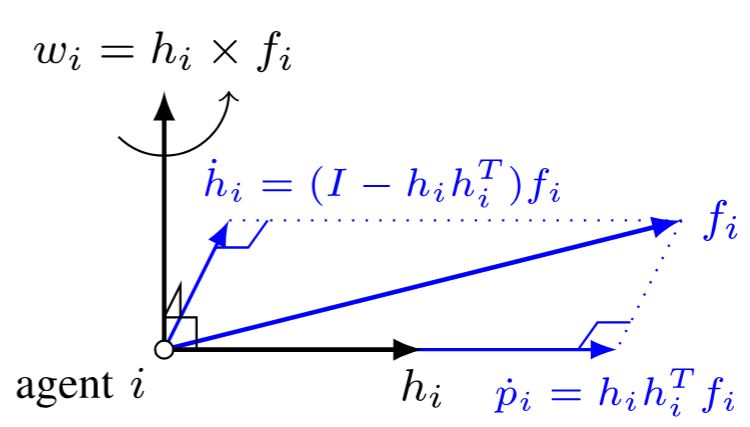
The geometric interpretation of $(2.2)$ is that ${\mathit{w}}_i$ attempts to rotate ${\mathit{h}}_i$ to align with ${\mathit{f}}_i$ (see Figure 2.1 for an illustration). Denote $[\cdot {]}_{\times }$as the skew-symmetric matrix of a vector. For any $\mathit{x}={[x_1,x_2,x_3]}^{\mathrm{\top }}\in {\mathbb{R}}^3$

$$[\mathit{x}{]}_{\times }:=\left[\begin{array}{lll}0& -x_3& x_2\\ x_3& 0& -x_1\\ -x_2& x_1& 0\end{array}\right]$$

Then, we have $\mathit{x}\times \mathit{y}=[\mathit{x}{]}_{\times }\mathit{y}$ for any $\mathit{x},\mathit{y}\in {\mathbb{R}}^3$. Substituting $(2.2)$ into $(2.1)$ gives

$${\dot{\mathit{h}}}_i=-{\left[{\mathit{h}}_i\right]}_{\times }{\mathit{w}}_i=-{\left[{\mathit{h}}_i\right]}_{\times }^2{\mathit{f}}_i=(\mathbf{I}-{\mathit{h}}_i{\mathit{h}}_i^{\mathrm{\top }}){\mathit{f}}_i$$

where the last equability follows from the fact that $-[\mathit{x}{]}_{\times }^2=\mathbf{I}-\mathit{x}{\mathit{x}}^{\mathrm{\top }}$ for any unit vector $\mathit{x}\in {\mathbb{R}}^3$. Then, the modified gradient control law $(2.1)$ becomes

$$\begin{array}{}\text{(2.3)}& \begin{array}{rl}& {\dot{\mathit{p}}}_i={\mathit{h}}_i{\mathit{h}}_i^{\mathrm{\top }}{\mathit{f}}_i\\ & {\dot{\mathit{h}}}_i=(\mathbf{I}-{\mathit{h}}_i{\mathit{h}}_i^{\mathrm{\top }}){\mathit{f}}_i,i\in \mathcal{V}\end{array}\end{array}$$

Note that $\mathbf{I}-{\mathit{h}}_i{\mathit{h}}_i^{\mathrm{\top }}$ is an orthogonal projection matrix that projects any vector onto the orthogonal complement of ${\mathit{h}}_i$. Although derived in ${\mathbb{R}}^3$, control law $(2.3)$ is also valid in ${\mathbb{R}}^2$ because the case of ${\mathbb{R}}^2$ can be viewed as a special case of ${\mathbb{R}}^3$ by treating the plane spanned by ${\mathit{h}}_i$ and ${\mathit{f}}_i$ as the $X-Y$ plane in ${\mathbb{R}}^3$.

Figure 2.1: Illustration of the modified gradient control law in (2.3)[1].

The convergence of $(2.3)$ is analyzed as follows.

Theorem 1 (Modified Gradient Control Law)

Under Assumption 1, the modified gradient coordination control law $(2.3)$ is convergent with the same attraction region as $(1.1)$.

Proof:

Details of Proof

The error dynamics corresponding to $(2.3)$ is $\dot{\mathit{e}}=(\partial \mathit{e}/\partial \mathit{p})\mathbf{M}\mathit{f}$ where $\mathbf{M}=\mathrm{diag}({\mathit{h}}_1{\mathit{h}}_1^{\mathrm{\top }},\dots ,{\mathit{h}}_n{\mathit{h}}_n^{\mathrm{\top }})\in {\mathbb{R}}^{(dn)\times (dn)}$. The time derivative of $V$ is

$$\dot{V}=-\sum _{i\in \mathcal{V}}{\mathit{f}}_i^{\mathrm{\top }}{\dot{p}}_i=-\sum _{i\in \mathcal{V}}{\mathit{f}}_i^{\mathrm{\top }}{\mathit{h}}_i{\mathit{h}}_i^{\mathrm{\top }}{\mathit{f}}_i\le 0.$$

It follows that $\mathrm{\Omega }\left(V\left({\mathit{e}}_0\right)\right)\subseteq \mathrm{\Omega }\left(r_0\right)$ is positively invariant for any ${\mathit{e}}_0\in \mathrm{\Omega }\left(r_0\right)$. Let $\mathcal{M}=\{\mathit{e}:\dot{V}(e)=0\}$. Then, the system trajectory starting from any point in $\mathrm{\Omega }\left(V\left({\mathit{e}}_0\right)\right)$ converges to the largest invariant set in $\mathcal{M}\cap \mathrm{\Omega }\left(V\left({\mathit{e}}_0\right)\right)$ by the invariance principle. For any point in $\mathcal{M}$, we have ${\mathit{h}}_i^{\mathrm{\top }}{\mathit{f}}_i=0$ for all $i$, which indicates either ${\mathit{f}}_i=0$ for all $i$ or ${\mathit{h}}_i\perp {\mathit{f}}_i$ but ${\mathit{f}}_i\ne 0$ for certain $i$. In the first case, it follows that $e=0$ by condition 2) in Assumption 1. As a result, the error converges to zero and the theorem is proved. The second case is impossible. To see that assume ${\mathit{h}}_i\perp {\mathit{f}}_i$ but ${\mathit{f}}_i\ne 0$. Then, ${\dot{p}}_i={\mathit{h}}_i{\mathit{h}}_i^{\mathrm{\top }}{\mathit{f}}_i=0$ for all $i$, which indicates that all the agents are stationary. As a result, ${\mathit{f}}_i$ is time invariant for all $i$. However, it follows from ${\mathit{h}}_i\perp {\mathit{f}}_i$ that ${\dot{h}}_i=(\mathbf{I}-{\mathit{h}}_i{\mathit{h}}_i^{\mathrm{\top }}){\mathit{f}}_i={\mathit{f}}_i\ne 0$. As a result, ${\mathit{h}}_i$ is rotating. It is impossible to maintain ${\mathit{h}}_i\perp {\mathit{f}}_i$ if ${\mathit{f}}_i$ is time invariant while ${\mathit{h}}_i$ is rotating. Hence, the system trajectory will escape from $\mathcal{M}$.

Theorem 1 indicates that if $\mathrm{\Omega }\left(r_0\right)$ is the attraction region of the gradient system $(1.1)$, then it remains an attraction region for the modified gradient system $(2.3)$. As a result, if the original gradient control is globally (respectively, locally) stable, then the modified one is also globally (respectively, locally) stable. The initial values of the heading vectors ${\{{\mathit{h}}_i(0)\}}_{i\in \mathcal{V}}$ do not affect the convergence. The final values ${\{{\mathit{h}}_i(\mathrm{\infty })\}}_{i\in \mathcal{V}}$ are not specified.

B. Application to Unicycle Models

Considering that unicycle models have been widely considered in multiagent coordination control, we apply $(2.3)$ to derive the specific control law for unicycle agents moving in the plane. It is, however, worth noting that $(2.3)$ is applicable to agents moving in both two and three dimensions.

Let ${\mathit{p}}_i={[x_i,y_i]}^{\mathrm{\top }}\in {\mathbb{R}}^2$ and ${\theta }_i\in \mathbb{R}$ be the position coordinate and heading angle of agent $i$, respectively. The motion of agent $i$ is governed by the unicycle model

$$\begin{array}{}\text{(2.4)}& \begin{array}{rl}& {\dot{x}}_i=v_i\cos {\theta }_i\\ & {\dot{y}}_i=v_i\sin {\theta }_i\\ & {\dot{\theta }}_i=w_i\end{array}\end{array}$$

where $v_i\in \mathbb{R}$ and $w_i\in \mathbb{R}$ are the linear and angular velocities. We propose the following control law for the unicycle model

$$\begin{array}{}\text{(2.5)}& \begin{array}{rl}{v}_i& =[\cos {\theta }_i,\sin {\theta }_i]{\mathit{f}}_i\\ w_i& =[-\sin {\theta }_i,\cos {\theta }_i]{\mathit{f}}_i\end{array}\end{array}$$

The convergence of the control law is proved below.

Theorem 2 (Control Law for Unicycle Agents)

Under Assumption 1, control law $(2.5)$ designed for the unicycle model in $(2.4)$ is convergent with the same attraction region as $(1.1)$.

Proof:

Details of Proof

Let ${\mathit{h}}_i={[\cos {\theta }_i,\sin {\theta }_i]}^{\mathrm{\top }}$ and ${\mathit{h}}_i^{\perp }={[-\sin {\theta }_i,\cos {\theta }_i]}^{\mathrm{\top }}$. Note that ${\mathit{h}}_i\perp {\mathit{h}}_i^{\perp }$. Substituting control law $(2.5)$ into the unicycle model yields ${\dot{p}}_i={\mathit{h}}_i{\mathit{h}}_i^{\mathrm{\top }}{\mathit{f}}_i$ and ${\dot{h}}_i={\mathit{h}}_i^{\perp }{\left({\mathit{h}}_i^{\perp }\right)}^{\mathrm{\top }}{\mathit{f}}_i$. Since ${\mathit{h}}_i^{\perp }{\left({\mathit{h}}_i^{\perp }\right)}^{\mathrm{\top }}=I-{\mathit{h}}_i{\mathit{h}}_i^{\mathrm{\top }}$, the closed-loop system has the same expression as $(2.3)$. The convergence property then follows from Theorem 1.

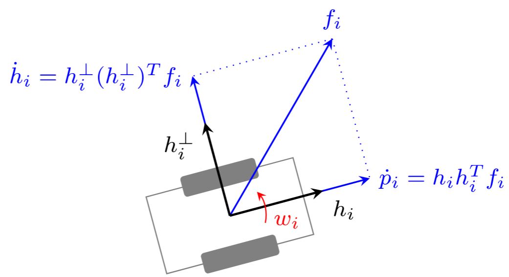
The geometric interpretation of the control law in $(2.5)$ is illustrated in Figure 2.2. The initial values of the heading angles ${\{{\theta }_i(0)\}}_{i\in \mathcal{V}}$ do not affect the convergence. The final values ${\{{\theta }_i(\mathrm{\infty })\}}_{i\in \mathcal{V}}$ are not specified. We next apply $(2.5)$ to derive a displacement-based formation control law for unicycles.

Figure 2.2: Geometric interpretation of the control law in (2.5). Note that p _i is the orthogonal projection of f_i onto h_i and \dot{h}_i is the orthogonal projection of f_i onto h_i^⊥. The angular velocity aims to turn h_i to align with f_i[1].

Example 2 (Displacement-Based Formation Control of Unicycles)

Consider the displacement-based formation control law ${\dot{p}}_i={\mathit{f}}_i=\sum _{j\in {\mathcal{N}}_i}({\mathit{p}}_j-{\mathit{p}}_i-{\mathit{p}}_j^{\ast }+{\mathit{p}}_i^{\ast })$. Substituting ${\mathit{f}}_i$ into $(2.5)$ yields

$$\begin{array}{}\text{(2.6)}& \begin{array}{rl}{v}_i& =[\cos {\theta }_i,\sin {\theta }_i]\sum _{j\in {\mathcal{N}}_i}({\mathit{p}}_j-{\mathit{p}}_i-{\mathit{p}}_j^{\ast }+{\mathit{p}}_i^{\ast })\\ w_i& =[-\sin {\theta }_i,\cos {\theta }_i]\sum _{j\in {\mathcal{N}}_i}({\mathit{p}}_j-{\mathit{p}}_i-{\mathit{p}}_j^{\ast }+{\mathit{p}}_i^{\ast })\end{array}\end{array}$$

Another well-known formation control law for unicycles proposed in [1, eq. $(1.1)$] is

$$\begin{array}{}\text{(2.7)}& \begin{array}{rl}& v_i=[\cos {\theta }_i,\sin {\theta }_i]\sum _{j\in {\mathcal{N}}_i}({\mathit{p}}_j-{\mathit{p}}_i-{\mathit{p}}_j^{\ast }+{\mathit{p}}_i^{\ast })\\ & w_i=\cos t\end{array}\end{array}$$

The two control laws in $(2.6)$ and $(2.7)$ have the same linear velocity. They, however, have different angular velocities. The angular velocity in $(2.7)$ $w_i=\cos t$ will cause periodical rotation of the unicycle. When compared, the control law in $(2.6)$ is more reasonable in the sense that it avoids unnecessary periodical rotations by turning the heading vector to align with the gradient flow.

Example 3: Displacement-Based Formation Control

The objective of displacement-based formation control is to steer the agents from some initial positions to converge to a desired geometric pattern defined by constant relative positions ${\{{\mathit{p}}_i^{\ast }-{\mathit{p}}_j^{\ast }\}}_{(i,j)\in \mathcal{E}}$. This formation control problem degenerates to the rendezvous problem when ${\mathit{p}}_i^{\ast }={\mathit{p}}_j^{\ast }$ for all $i,j\in \mathcal{V}$. Consider the Lyapunov function

$$V=\frac{1}{4}\sum _{i\in \mathcal{V}}\sum _{j\in {\mathcal{N}}_i}{\Vert ({\mathit{p}}_i-{\mathit{p}}_j)-({\mathit{p}}_i^{\ast }-{\mathit{p}}_j^{\ast })\Vert }^2.$$

The target formation is achieved if and only if $V=0$ since the graph is bidirectional and connected. The gradient control law

$$\dot{{\mathit{p}}_i}={\mathit{f}}_i=\sum _{j\in {\mathcal{N}}_i}[({\mathit{p}}_j-{\mathit{p}}_i)-({\mathit{p}}_j^{\ast }-{\mathit{p}}_i^{\ast })]$$

is the displacement-based formation control law. Consider any oriented graph and define the error state as ${\mathit{e}}_k={\mathit{p}}_i-{\mathit{p}}_j-({\mathit{p}}_i^{\ast }-{\mathit{p}}_j^{\ast })$ with $k=1,\dots ,m$ and $\mathit{e}=(\mathbf{H}\otimes \mathbf{I})(\mathit{p}-{\mathit{p}}^{\ast })$. Then, $V(\mathit{e})=1/2\sum _{i=1}^m{\Vert {\mathit{e}}_k\Vert }^2,\partial \mathit{e}/\partial \mathit{p}=\mathbf{H}\otimes \mathbf{I}$ is constant, $\mathit{f}$ is continuous in $\mathit{e}$, and $\parallel \mathit{f}\parallel$ is bounded when $\parallel \mathit{e}\parallel$ is bounded. Since $V=1/2{(\mathit{p}-{\mathit{p}}^{\ast })}^{\mathrm{\top }}(L\otimes \mathbf{I})(\mathit{p}-{\mathit{p}}^{\ast })$ and $\dot{p}=\mathit{f}=-(L\otimes \mathbf{I})(\mathit{p}-{\mathit{p}}^{\ast })$, we have $\mathit{f}=\mathbf{0}\iff V=0\iff \mathit{e}=\mathbf{0}$ and the attraction region $\mathrm{\Omega }\left(r_0\right)$ is the entire space ${\mathbb{R}}^{dm}$. Therefore, all the conditions in Assumption 1 are satisfied.

Example 4: Bearing-Based Formation Control

The objective of bearing-based formation control is to steer the agents from some initial positions to converge to a desired geometric pattern defined by constant interneighbor bearings ${\left\{{\mathit{g}}_{ij}^{\ast }\right\}}_{(i,j)\in \mathcal{E}}$. Consider the Lyapunov function

$$V=\frac{1}{4}\sum _{i\in \mathcal{V}}\sum _{j\in {\mathcal{N}}_i}{\Vert {\mathit{p}}_{{\mathit{g}}_{ij}^{\ast }}({\mathit{p}}_i-{\mathit{p}}_j)\Vert }^2$$

where ${\mathit{p}}_{{\mathit{g}}_{ij}^{\ast }}=\mathbf{I}-{\mathit{g}}_{ij}^{\ast }{\left({\mathit{g}}_{ij}^{\ast }\right)}^{\mathrm{\top }}$. The gradient control law

$$\dot{{\mathit{p}}_i}={\mathit{f}}_i=\sum _{j\in {\mathcal{N}}_i}{\mathit{p}}_{{\mathit{g}}_{ij}^{\ast }}({\mathit{p}}_j-{\mathit{p}}_i)$$

is the bearing-based formation control law. For any oriented graph, define the error state as ${\mathit{e}}_k={\mathit{p}}_{{\mathit{g}}_{ij}^{\ast }}({\mathit{p}}_i-{\mathit{p}}_j)$ with $k=1,\dots ,m$. Then, $V(\mathit{e})=1/2\sum _{k=1}^m{\Vert {\mathit{e}}_k\Vert }^2,\partial \mathit{e}/\partial \mathit{p}=\mathrm{diag}({\mathit{p}}_{{\mathit{g}}_1^{\ast }},\dots ,{\mathit{p}}_{{\mathit{g}}_m^{\ast }})(\mathbf{H}\otimes \mathbf{I})$ is constant, $\mathit{f}$ is uniformly continuous in $\mathit{e}$, and $\parallel \mathit{f}\parallel$ is bounded when $\parallel \mathit{e}\parallel$ is bounded. Let $L_{\mathcal{B}}\in {\mathbb{R}}^{dn\times dn}$ be the bearing Laplacian. Then, $V=1/2{\mathit{p}}^{\mathrm{\top }}{L}_{\mathcal{B}}\mathit{p}$ and $\dot{\mathit{p}}=\mathit{f}=-L_{\mathcal{B}}\mathit{p}$. As a result, $\mathit{f}=\mathbf{0}\iff V=\mathbf{0}\iff \mathit{e}=\mathbf{0}$ and the attraction region $\mathrm{\Omega }\left(r_0\right)$ is the entire space ${\mathbb{R}}^{dm}$. Therefore, all the conditions in Assumption 1 are satisfied.

References

1. Shiyu Zhao, D. V. Dimarogonas, Zhiyong Sun, and D. Bauso, A General Approach to Coordination Control of Mobile Agents With Motion Constraints, IEEE Transactions on Automatic Control, vol. 63, no. 5, pp. 1509–1516, May 2018: Section II & III, Appendix.

---

1. A function $f(x)$ is uniformly continuous in $x$ if for any $\epsilon >0$ there exists $\delta >$ 0 such that $\Vert f\left(x_1\right)-f\left(x_2\right)\Vert <\epsilon$ for every pair of $x_1$ and $x_2$ satisfying $\parallel x_1-x_2\parallel <\delta$. A sufficient (yet not necessary) condition for uniform continuity is that if a function is differentiable and its derivative is bounded, then the function is uniformly continuous. This sufficient condition will be frequently used in the proof of Theorem 3. ↩︎