Basis
- Rigid graph control architectures for autonomous formations by D. O. Anderson etc.;
- Section 1.2-1.3 of Formation Control of Multi-Agent Systems: A Graph Rigidity Approach by Marcio de Queiroz etc.;
- Theorem from Conditions for unique graph realizations by Bruce Hendrickson;
- Preliminaries part of Distributed estimation and control for preserving formation rigidity for mobile robot teams by Zhiyong Sun, ..., D. O. Anderson;
- Preliminaries part of Distributed stabilization control of rigid formations with prescribed orientation by Zhiyong Sun, ..., D. O. Anderson, Hyo-Sung Ahn
Graph Theory
Please make sure you are familiar with the concept of graph
Consider an undirected graph with
Definition: complete graph
A graph
Definition: path
A path is a trail that goes from an origin vertex to a destination vertex by traversing edges of the graph.
Definition: connected
Two vertices
- the vertex set: the robots (and we may use the word agent interchangeably in the context)
- the edge set: the communication links between different robots
The incidence matrix:
For a connected and undirected graph, one has:
.
The adjacency matrix:
The Laplacian matrix:
Lemma Properties of Laplacian matrix
is orientation-independent is symmetric and positive semidefinite - If
is connected, then has one and only one zero eigenvalue, with where is a column vector
Definition: induced subgraph
For a graph
Framework
Definition: Framework
A framework is simply a realization of a graph at given points in Euclidean space. Specifically, if
The importance of a framework is that it can model a physical structure. That is, consider the so-called “bar-and-joint” framework, which is a structure made of rigid bars joined at their ends by universal joints. A bar-and-joint framework can be used to describe a wide range of static and dynamic structures, such as bridges, mechanical linkages, and biological molecules.
In 2D, treat
with
Introduce:
denote block diagonal matrix of the relative position.
The edge function (Specific for distance rigidity function denoted as
where the norm is the standard Euclidean norm, and the
Rigidity Theory
Rigidity Graphs
Characterized by rigid body
Given a bar-and-joint framework, a fundamental question is whether it is rigid or not. By rigidity, we mean the non-deformation of the structure.
Roughly speaking, a formation is rigid if its only smooth motions are those corresponding to translation or rotation of the whole formation
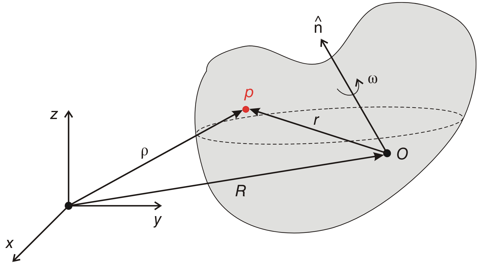
Definition: Translation and Rotation of a rigid body
A rigid body is said to be in translation if all points forming the body move along parallel paths (straight or curvilinear). A rigid body is said to be in rotation if all points move in parallel planes along circles centered on a same axis that intersects the body.
If the axis of rotation does not intersect the rigid body, the motion is usually called a revolution or orbit. This type of motion (in fact, any type of rigid body motion) can be decomposed into a translation superimposed on a rotation. That is, the above definitions allow one to decouple pure translation from pure rotation. Recall from rigid body kinematics that given body-fixed points
where
Definition: Equivalent & Congruent
Two frameworks
- Equivalent: if
for all , i.e., the edge function (2) is the same; - Congruent: if
for all (with ), i.e., all distances between vertices are the same (such pairs is always );
Note that congruency implies equivalency, but the reverse is not necessarily true.
Definition: isometry
An isometry of
Note that
Two frameworks
Definition
A motion of a framework
This leads us to the following definition of rigidity.
Definition: rigidity
A framework
On the other hand, the framework is flexible in
Chacaterized in Combination
Counting-type conditions related to the graph can be used to ascertain the rigidity or nonrigidity of a generic formation corresponding to the graph.
Laman's Theorem
A graph
If a graph
- there exists a subgraph
with edges such that, for every subset of , the induced subgraph of satisfies - if
, then is 3-connected (equivalently, every pair of vertices of is connected by three paths that pairwise have no vertices in common except the end vertices).
Characterized in Linear Algebra
First, embed the graph
Definition: (global) rigidity
A framework
Two frameworks
Infinitesimal Rigidity
Although our physical intuition can indicate if certain frameworks are rigid or not, in general it is difficult to determine rigidity from the definition characterized by rigid body. Therefore, we will consider a related notion of rigidity called infinitesimal rigidity, which can be easily verified via a matrix rank.
In general, rigidity does not imply infinitesimal rigidity, but infinitesimal rigidity implies rigidity. Frameworks that are rigid but not infinitesimally rigid usually have collinear or parallel edges.
For so-called generic frameworks, rigidity is equivalent to infinitesimal rigidity. When a framework
For example, The planar framework in Figure below is nongeneric in
In infinitesimal rigidity, instead of preserving distances during a continuous deformation, we require first-order preservation of distances during an infinitesimal motion. Therefore, infinitesimal rigidity (also called first-order rigidity) is a linear approximation to rigidity.
In the definition of continuous family, i.e. formula
where
where
When analyzing infinitesimal rigidity, the rigidity matrix of a framework comes in handy, which is defined as
Note that:
- the entries of
only involve relative position vectors , and we can rewrite it as . - the rigidity matrix has a row for each edge and
columns for each vertex. That is, for the -th edge of connecting vertices and , the -th row of is where is in the columns for vertex , is in the columns for vertex , and all other elements are zero.
A useful structural property of the rigidity matrix:
given any vector
Using
where
Let
Note that if a framework undergoes any rigid body motion, then according to
where
Notice that the vectors are defined here with dimension
irrespective of the Euclidean space of the framework. If the framework is planar, then .
It is not difficult to check that
upon use of the properties of vector products. In other words, rigid body motions produce infinitesimal motions. This leads us to the following definition.
Definition: infinitesimal rigidity
A framework is infinitesimally rigid if the only solutions to
We can use Definition above to determine if a framework is infinitesimally rigid or flexible by attempting to assign a velocity vector to each vertex such that
Fortunately, there is an easy way of checking whether a framework is infinitesimally rigid via the rank of the rigidity matrix. Before presenting this useful result, we need the following facts:
- the rank of an
matrix is equal to minus the dimension of its null space. - the number of independent rigid body motions for a generic framework in
is . This means that there exist independent rigid body motions in (translation along , translation along , and rotation about ) and in (translations along and rotations about ).
Given the above, we deduce that
Theorem 1
Consider a framework
Obviously, in order to have an infinitesimally rigid framework, the graph should have at least
From Theorem 1, one knows that the dimension of the null space of
Lemma 1: Null space of the rigidity matrix
Suppose the framework
: The null space of is of dimension and is described as , where
and the matrix
: The null space of is of dimension and is described as , where
and the matrix
TODO Proof
Lemma 2
Suppose the framework
TODO Proof
- if
is infinitesimally rigid, so is for a generic (open and dense) set of . - Generally speaking, infinitesimal rigidity implies rigidity, but the converse is not true.
As discussed earlier, the rigidity property of a generic framework
Theorem 2
Consider two frameworks
Here,
Proof: Let
Obviously,
Minimal Rigidity
It is obvious that adding edges to a graph does not destroy rigidity. A natural question is then: What is the minimum number of edges that ensures rigidity? This is important in practice because it ensures that a formation of multiple agents is rigid with the minimum number of sensing and communication links. The disadvantage of minimal rigidity is that it lacks robustness to the loss of a sensor or communication link since redundant edges are removed from the graph
Definition: minimally rigidity
A formation is minimally rigid if it is rigid and if no single interagent distance constraint can be removed without causing the formation to lose rigidity
A graph is minimally rigid if almost all formations to which the graph corresponds are minimally rigid.
As for minimal rigidity, it can be described in 2D and 3D with the rigidity matrix, is characterizable in 2D with Laman’s theorem, and, in 3D, is the subject of necessary conditions and distinct sufficiency conditions on the graph determined by a formation.
Given a graph with edge set
Theorem 3
A rigid graph is minimally rigid if and only if
This leads to the following corollary.
Corollary 1
If a framework is infinitesimally and minimally rigid, then its rigidity matrix has full row rank and
Proof: Given that the rigidity matrix has
Note that
Henneberg construction
The Henneberg construction deals with the iterative construction of rigid formations. As for the characterization of rigidity, the Henneberg construction procedure for 2D formations is better developed than that for 3D formations.
The 2D Henneberg construction comprises the application at each step of one of two possible operations, known as vertex addition and edge splitting.
The procedure begins with a minimally rigid graph, and the application of either operation creates a minimally rigid graph with one additional vertex. Minimally rigid graphs can be progressively built up this way
Definition: Henneberg Construction
The Henneberg construction is a technique for growing minimally rigid graphs, starting from a graph with two vertices and one edge joining the vertices.
At each step in the procedure, illustrated in greater detail below, either a vertex and two edges are added, or a vertex and three new edges are added, while one existing edge is removed. The new edges are incident on the new vertex. These operations are termed vertex addition and edge splitting, respectively.
vertex addition Let
be a graph modeling a formation in 2D. A new graph is formed, where a vertex v is adjoined as well as two edges from to , so that and for some . edge splitting A new graph
is formed from , where and for some with at least two of the vertices adjacent in , and the edge either , or
These vertex-addition and edge-splitting operations are enough to grow every minimally rigid graph. It is also possible to deconstruct a minimally rigid graph by removing one vertex and a net count of two edges at each step
In growing and deconstructing a minimally rigid graph, all the intermediate graphs are minimally rigid
A by-product is the fact that every 2D minimally rigid graph is constructible from a primitive comprising a two-vertex single edge graph by using a sequence of these operations
In 3D, operations that are analogous to vertex addition and edge splitting can be defined, but whether these analogously defined operations are necessary and sufficient to build and deconstruct all minimally rigid graphs is still a matter of conjecture
Framework Ambiguities
Consider that a graph
- flip ambiguity: one vertex can be flip to another side. This occurs when a graph in
has a set of vertices lying in a -dimensional subspace about which a portion of the graph can be reflected. Notice that there cannot be any edges between the portions of the graph separated by the mirror edge. - Not every minimally rigid graph contains a flip ambiguity
- Multiple flips can happen in a given framework
- discontinuous flex ambiguity: positions of 2 or more vertexes can be changed while satisfying the constraints. This occurs in minimally rigid graphs since the removal of an edge allows a portion of the graph to flex. If the removed edge is reinserted after a flexing, one may obtain an equivalent framework with a different configuration.
- Every formation corresponding to a minimally rigid graph with four or more vertices at generic positions can exhibit flex ambiguity
This leads us to the following definition.
Definition: ambiguous
If two infinitesimally rigid frameworks are equivalent but not congruent, then they are said to be ambiguous.
We denote the set of all ambiguities of an infinitesimally rigid framework
The existence of framework ambiguities is problematic for formation control since the control law cannot distinguish the actual framework from an ambiguous one if only the edge lengths (i.e., inter-agent distances) are being controlled. In such a case, one solution is to initialize the agents sufficiently close to the desired framework to avoid their convergence to an ambiguous framework. From a control theory standpoint, this means that stability results will be local in nature rather than global. The following corollary to Theorem 2 will be helpful in establishing the stability.
Corollary of Theorem 2
Let
If
Proof: First, note that
Globally Rigidity
Consider a formation with distinctly labeled agents and with some of the interagent distances known. We wish to understand what alternative formation shapes agents can have when they are positioned consistently with the data. Note that if the formation
Deifnition: globally rigidity
A 2D or 3D formation is globally rigid if and only if one of the following works:
- any two formations corresponding to the distance data differ by a combination of translation, rotation, and reflection
- every framework that is equivalent to
is congruent to shown in the definition of rigidity.
A graph is globally rigid if and only if a generic formation corresponding to the graph is globally rigid.
Global rigidity is a more demanding concept than rigidity since there exist rigid formations that are not globally rigid, and such formations can be converted to globally rigid formations only by the inclusion of additional distance constraints.
- Local rigidity: cannot cannot deform smoothly from one shape. Minimal rigidity therefore allows retention of shape only in the face of potential smooth deformations, although it does not of itself specify what shape is retained. But with same constraints, graph can have different shapes
- Global rigidity: ensure that the shape is unique
A nice characterization of global rigidity is available for 2D formations and their associated graphs. No extension is known for 3D formations. The 2D characterization uses the terms redundant rigidity and three connectivity.
Definition: redundant rigidity
An undirected graph is termed redundantly rigid if it remains rigid after the removal of any single edge.
Definition: connected graph
A graph is connected if there is a path from any vertex to any other vertex. A graph is
Theorem 4
A graph
- When a graph is globally rigid, a generic formation corresponding to the graph is also globally rigid.
- A variation of Laman’s theorem is available that characterizes the redundant rigidity property.
- A useful property of a 2D globally rigid formation is that if the positions of three noncollinear agents are known, then the positions of all the other agents can be uniquely determined from the interagent distances corresponding to the edges in the formation graph.
Application:
- sensor network localization: unit disk graph use the distance data to determine the Euclidean coordinates for the sensor positions that are consistent with the distance set. The Euclidean coordinates, however, become uniquely specified by using further information obtained from designated anchor nodes or sensors, whose positions are known absolutely
Globally rigid formations with four or more agents are not minimally rigid. A reason for using nonminimally rigid formations, where more constraints are imposed than are needed for shape maintenance: loss of a sensor / communication link / control actuator
Some problems arise in handling nonminimally rigid formations: if the distances between agents in a formation are measured with some noise and controls operate to try to bring certain distances to specified values, a similar type of inconsistency will be likely to arise
Formations
The task of maintaining a prescribed distance between a pair of agents requires control action. The execution of the task could be the responsibility of both agents or one nominated agent of the pair.
- Modeling using undirected graphs is appropriate in the case of shared responsibility
- The case of single-agent or unilateral responsibility is captured by assigning a direction to the relevant edge in the graph
A directed edge from vertex
Therefore, and advantageously, both the overall communication complexity in terms of sensed or received information and the overall control complexity for the formation are halved in comparison to the shared responsibility case.
The reduction in communication links can mean lower bit rates and reduced difficulties with interference. In the shared responsibility case, a problem can arise when noise is present and two agents fail to share distance estimate information and instead use inconsistent estimates of the distance between each other, but this problem cannot arise in the single-agent responsibility case
Constraint Consistence and Persistence of Formations
Consider conditions involving unilateral distance constraints that ensure that the motions of a formation are restricted to translations or rotations of the formation as a whole.
A notion of persistence is introduced, which is an amalgam of two conditions, specifically, rigidity and a further notion of constraint consistence.
- Rigidity: if certain interagent distances are maintained, then all interagent distances are maintained when the formation moves smoothly
- Constraint consistence: the ability to maintain the specified interagent distances
- NOT constraint consistence: When one agent moves, another agent has an impossible task due to the former agent is unconscious of the constraint
- A 2D graph that has no more than 2 outgoing edges from every vertex is constraint consistent, although there are constraint consistent graphs that possess vertices having out-degree greater than two
A graph can be checked for persistence, that is, rigidity plus constraint consistence, by testing a certain collection of subgraphs for rigidity:
In 2D, Let
In 3D, the same idea applies, except that outgoing edges in excess of
Securing Persistence
Suppose that a 2D undirected graph is rigid. Can we assign edge directions so that it is constraint consistent and thus persistent? The question in its full generality remains open. However, affirmative answers exist for minimally rigid graphs, as well as for graphs with certain structures, including wheel graphs, trilateration graphs, complete graphs, and power graphs of cycle graphs
See Acquiring and maintaining persistence of autonomous multi-vehicle formations for more details
The simplest algorithm for assigning directions in a minimally rigid graph is to consider the associated undirected graph and determine a Henneberg sequence that generates it. Then directions can be assigned to the edges that are added at each step, using the rule that any vertex can have no more than two outgoing edges. Such a directed graph is termed minimally persistent. Minimally persistent graphs are precisely those that are minimally rigid and constraint consistent.
Figure 3 shows some direction assignments for wheel graphs and C
Wheel and C
Henneberg Sequence Theory and Persistent Graphs
The broad conclusion is that the technique can be applied, so long as the primitive operations are modified to allow directed edges in the graphs, and also a further primitive operation is introduced.
More than one operation is possible, with the simplest possible operation being edge-reversal, that is, reversing the direction of one edge arriving at a vertex that has
Definition: degree of freedom(DoF)
In 2D, a vertex is said to have
Extension of the Persistence Concept to 3D Formations
In 3D, most of the consistence and persistence ideas described above carry through. However, these extensions involve the behavior of subsets of agents, as opposed to individual agents or vertices. For
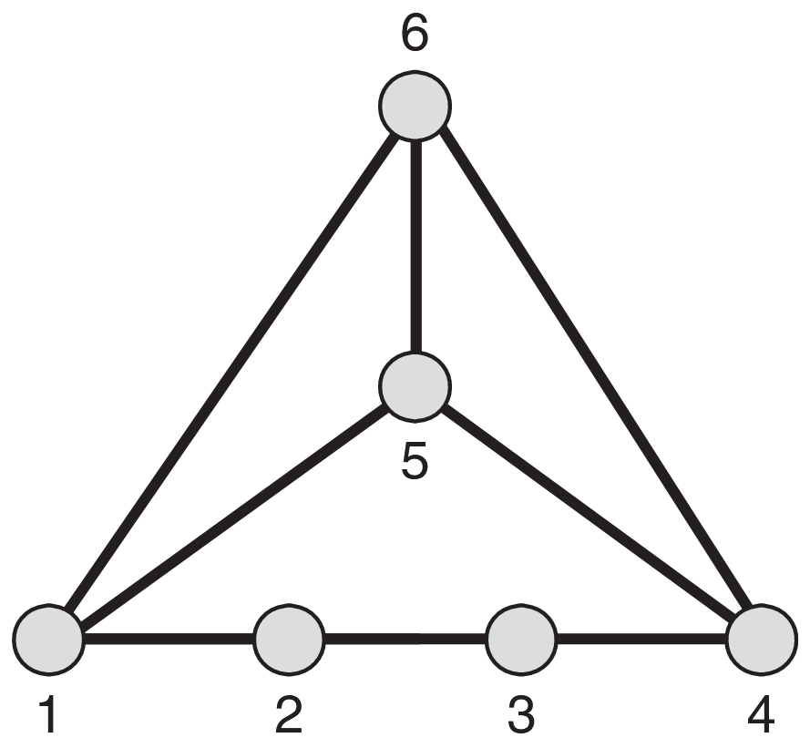
In 3D, checking structural persistence is trivial once persistence has been established. To illustrate structural persistence, Figure 4 depicts a 3D formation with an underlying directed graph, which is persistent since it is rigid and each agent has no more than three outgoing edges. However, agents 1 and 2 are unconstrained, having no outgoing edges, and so in principle can move apart, thus destroying the shape of the formation. Hence, despite the persistence property, this formation is not structurally persistent, and thus does not have a sensing and control architecture that allows retention of its shape
Every 3D graph that has no more than
In particular, the graph is structurally persistent if it is persistent and there is at most
If a graph is acyclic and persistent, it has at most
Operation with formations
Various operations on formations can be contemplated. In particular, the concepts of splitting, merging, and closing ranks are defined for formations that are modeled using undirected graphs.
An application domain where such scenarios arise is terrain surveillance and target localization using a formation of aerial vehicles. The individual vehicles carry sensors performing tasks such as range determination, bearing determination, or time-difference-of-arrival determination.
- In this application, acquiring and maintaining certain formation shapes and hence rigidity is essential because of the need for well-established coordination as well as optimality of certain formation geometries for cooperative localization. Formation shape maintenance within a class of allowable shapes may also be required in scenarios such as avoidance of obstacle collision or of entry into no-fly zones; this may be achieved by splitting, and merging back the split formations once the obstacle or no-fly zone is passed.
- Formation shape adjustment may also be needed for restructuring (closing ranks) to maintain rigidity and form an allowable shape in the event of loss of one or more aerial vehicle agents, or for addition of one or more aerial vehicle agents during a mission to improve surveillance coverage.
Apart from rigidity preservation, the successful execution of these maneuvers requires detailed consideration of agent dynamics (since instantaneous changes of control strategy can produce undesired transient behavior), as well as inclusion of collision-avoidance protection
Splitting
Consider a single rigid formation. Splitting refers to the division of the set of agents into two subsets, along with suppression of the distance constraints between agent pairs when the agents are in different subsets. Reasons for splitting include a change of objective or obstacle avoidance. See Figure 5 for an illustration of the problem.
In graph theory terms, the split yields two separate subgraphs, neither of which is guaranteed to be rigid. Introducing additional distance constraints in the separate subformations is thus required to ensure rigidity of each subformation separately.
Additionally, we could consider variations of the problem. For example, we could assume that the starting formation is minimally rigid, we could consider 2D and 3D formations, and we could consider directed graph versions. We could also consider algorithm complexity, as well as the possibility of imposing computational constraints on individual agents to perform calculations on a decentralized basis for determining where additional distance constraints should be inserted. These problems are largely open.
Merging
Consider two rigid formations. Merging requires the determination of additional distance constraints linking agent pairs with one agent drawn from each formation, such that the union of the agents of the two formations, along with the union of the distance constraints in the original formations and the new distance constraints, describes a single rigid formation. Figure 6 illustrates the problem.
Closing ranks
Consider a single rigid formation. Suppose that one agent is removed, and, consequently all distance constraints are lost between this agent and the remaining agents of the formation; see Figure 7.
The problem is to determine where new distance constraints can be inserted to recover rigidity. In addition, the closing ranks problem can be generalized to contemplate simultaneous removal of two or more agents from a formation, with the removal also of the associated distance constraints.
A technique is given below for dealing with the problems of splitting, merging and closing ranks.
Technique for dealing with operations
One way to solve these problems depends on a significant modification of the Henneberg sequence and is based on a minimal cover problem. This minimal cover problem presents a graph that is not rigid and for which a minimum number of new edges must be introduced to render the graph generically rigid. The solution of the minimal cover problem can be applied to solve the problems of formation merging, splitting, and closing ranks.
Additionally, the splitting problem is actually a particular case of the closing ranks problem, since one subformation can regard the agents of the other subformation as the lost agents. Further, the closing ranks problem can be solved by introducing new edges between former neighbors of the lost vertices of the graph, i.e., by performing a local repair as illustrated in Figure 7. Therefore, in the splitting problem, new edges can be restricted to connecting pairs of those vertices in one subformation graph that were previously neighbors of vertices that ended up in the other subformation graph, as illustrated in Figure 5.
The formation operations discussed above can also be contemplated for directed graphs
Metavertices, rigid bodies, and Metaformation
In merging two formations, much of the internal structure is largely irrelevant. For example, if two rigid formations are to be merged in 2D, the merging can be done by introducing
Rigidity and 2D Formations of Formations
Body-bar systems conceptually underpin the metaformation view of merging problems. A body is a generalization of a point agent. Any rigid formation of agents can be replaced by a body, a rigid object that in 2D has
A key problem is to determine when such a framework, better termed a metaformation given that it is obtained by interconnecting bodies, is rigid. Of course, we want to answer this problem without accounting for the internal structure of the bodies.
Rigidity is characterized for metaformations of bodies using both a generalization of the rigidity matrix and a generalization of Laman’s theorem for the 2D case. Recall that Laman’s theorem provides necessary and sufficient conditions for generic rigidity of a graph corresponding to a formation of point agents, and the conditions are of a counting form; a simple adjustment of certain numbers appearing in the statement of Laman’s theorem converts the result to a theorem concerning generic rigidity of a graph corresponding to a 2D bodyframework. However, as for checking rigidity of a normal graph in 3D, there is no known necessary and sufficient counting condition in the style of Laman’s theorem for a 3D body-bar framework to be rigid. On the other hand, the rigidity matrix ideas work in 3D space, where the bodies have
Interconnection of two formations involves the interconnection of two bodies, and the extension of Laman’s theorem states
More on Formation Merging
Besides the problem described above of connecting two formations in 2D, several other related problems can be considered:
- connecting, by means of insertion of additional edges, two formations in 3D to secure minimal rigidity
- connecting two formations in 2D / 3D to secure global rigidity
- connecting two formations when they are not disjoint. Nondisjoint formations may have a limited number of common vertices, or a limited number of common edges, or both.
By appealing to various results on rigidity and global rigidity, various conditions are established to solve these problems. These conditions require the insertion of a minimum or exactly specified number of new connections that are incident on a minimum specified number of vertices in each of the two merging formations. We give two examples to illustrate the results.
- Consider two globally rigid 2D graphs, with one vertex in common. By adding two new edges with one vertex in each formation, and such that in at least one of the formations the edges are incident on two distinct vertices, we obtain a globally rigid graph. Note that the two added edges cannot be incident on the vertex common to the two initially given graphs.
- Consider two minimally rigid graphs of 3D formations, with no vertices in common. Merging requires the addition of at least
new edges, with the new edge set incident in each graph on at least vertices. Most patterns involving precisely edges ensure that the merged graph is minimally rigid. Acceptable patterns include every pattern such that each graph has exactly vertices that the new edges are incident on. Each graph can have either new incident edges for each of the vertices, or edges incident on the vertices. A further set of patterns can be obtained using any vertex that has or more new incident edges, by moving one of those incidences to a new vertex in the same graph on which no new edge is yet incident. In this way, up to vertices in each of the two merging graphs can have a new edge incident on it. - A related result is that if the two 3D graphs are rigid but not necessarily minimally rigid, inserting
new edges using the same incidence rules yields a rigid graph. Such an interconnection can be regarded as minimally rigid from the metaformation point of view, since the issue of whether or not the individual metavertices are minimally rigid internally is irrelevant
- A related result is that if the two 3D graphs are rigid but not necessarily minimally rigid, inserting
Directed versions of these results are given in ref. Conditions for securing persistence include the conditions applicable to securing rigidity as discussed above. For example, to merge two minimally persistent graphs in 3D into a larger minimally persistent graph, we need to insert
If the merged graph must be persistent but not necessarily minimally persistent, we need to add
In 3D, if only two agents in the two persistent graphs have positive DoF, then the two graphs cannot be merged into a single persistent graph. However, in every other case, if at least
Figure 8 illustrates merging two persistent 2D formations using directed edges. As with undirected graphs, three new edges incident on at least two agents in each formation can achieve the merging. To ensure persistence of the overall structure, the vertices left by these three new edges must have in the merged structure a maximum out-degree of
For 3D formations, structural persistence of the merged formation is also desired. Requirements are set out in ref
Toward a More Systematic Theory
In 2D we have described a variation of Laman’s theorem describing the rigidity of a metaformation, obtained by connecting together metavertices or meta-agents. This result leads to the question of whether the concept of a Henneberg sequence can be extended to metaformations. Such a sequence could start with a single metavertex, or rigid formation, and involve the successive addition of meta-agents to the metaformation. Each addition would result in a metaformation that has the minimal number of edges between metavertices so as to guarantee rigidity of the overall metaformation. Indeed, such a construction is available. Analogues to the primitive operations of the standard Henneberg construction, namely, vertex addition and edge splitting, can be constructed. These operations are termed metavertex addition and metaedge splitting, respectively. See, for example, Figure 9. The construction can also be described by building on the results described in the previous section.